This document provides an overview of key concepts regarding normal distributions, including:
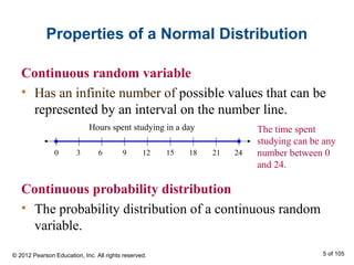
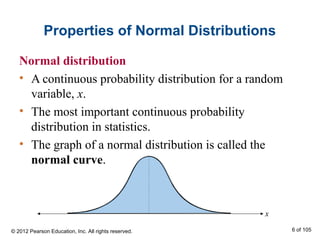
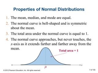
- Normal distributions have properties such as being bell-shaped and symmetric about the mean. The mean, median and mode are equal for a normal distribution.
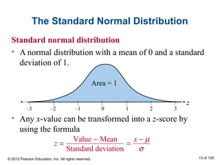
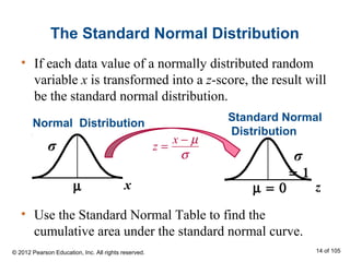
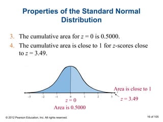
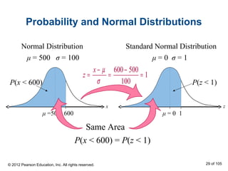
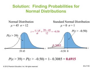
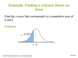
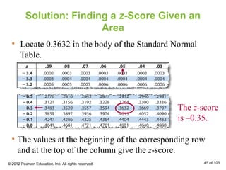
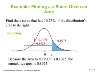
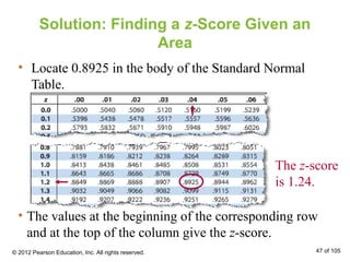
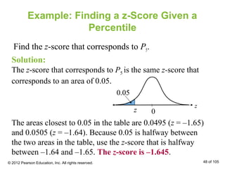
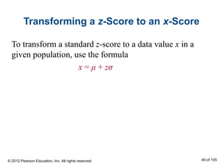
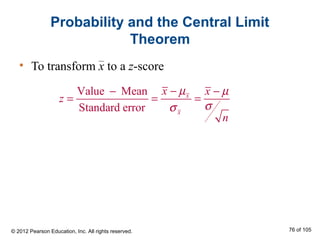
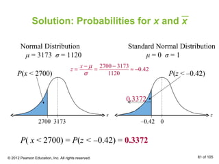
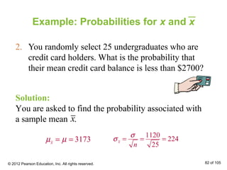
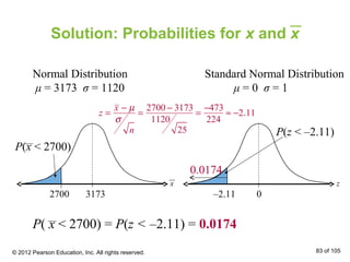
- The standard normal distribution has a mean of 0 and standard deviation of 1. Any normally distributed value can be converted to a z-score and related to the standard normal distribution.
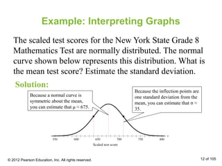
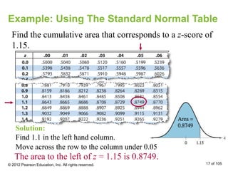
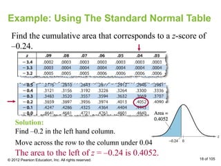
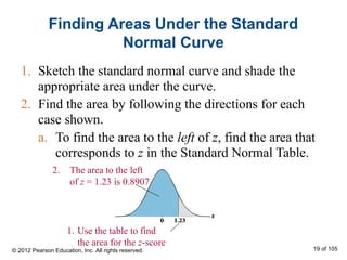
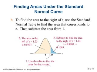
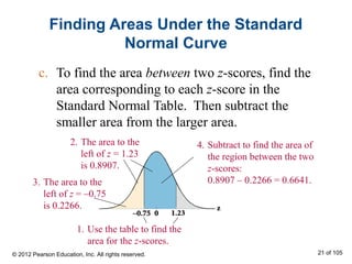
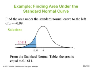
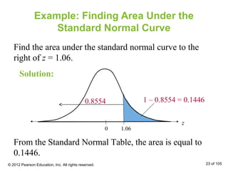
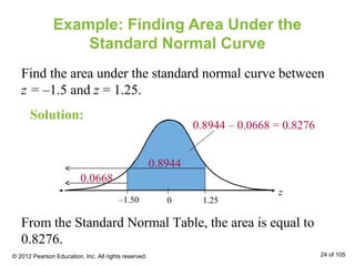
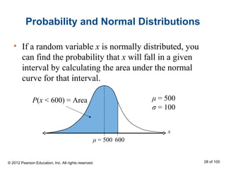
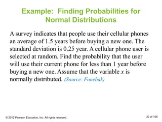
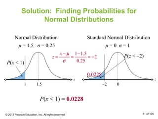
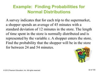
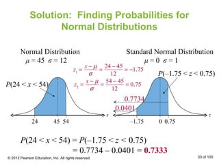
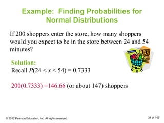
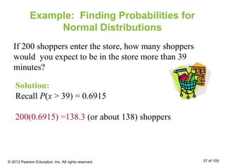
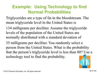
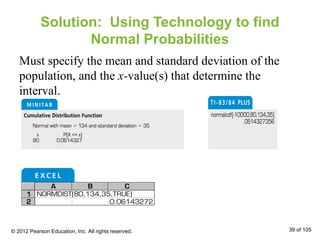
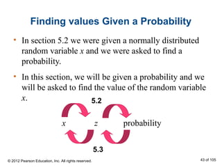
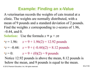
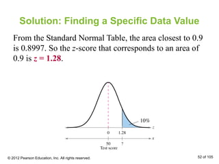
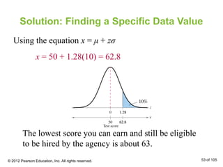
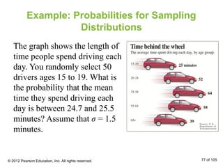
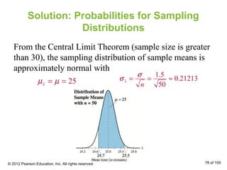
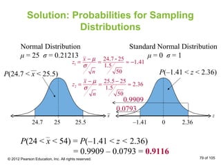
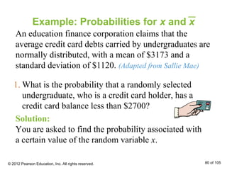
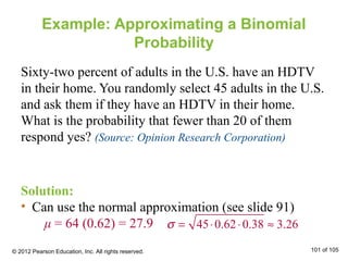
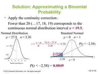
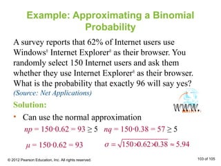
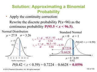
- Areas under the normal curve can be used to find probabilities for normally distributed variables. Specific examples are provided to demonstrate finding probabilities and related values.


![NORMAL DISTRIBUTION FIN [Autosaved].pptx](https://cdn.slidesharecdn.com/ss_thumbnails/normaldistributionfinautosaved-250706062357-4c5756a9-thumbnail.jpg?width=640&height=640&fit=bounds)


