Multimedia Communication Lec02: Info Theory and Entropy

CS/EE 5590 / ENG 401 Special Topics
(Class Ids: 17804, 17815, 17803)
Lec 02
Entropy and Lossless Coding I
Zhu Li
Z. Li Multimedia Communciation, 2016 Spring p.1
Outline
 Lecture 01 ReCap
 Info Theory on Entropy
 Lossless Entropy Coding
Video Compression in Summary
Video Coding Standards: Rate-Distortion Performance
 Pre-HEVC

PSS over managed IP networks
 Managed mobile core IP networks
MPEG DASH – OTT
 HTTP Adaptive Streaming of Video
Outline
 Self Info of an event
 Entropy of the source
 Relative Entropy
 Mutual Info
 Entropy Coding
Thanks for SFU’s Prof. Jie Liang’s slides!
Entropy and its Application
Entropy coding: the last part of a compression system
Losslessly represent symbols
Key idea:
 Assign short codes for common symbols
 Assign long codes for rare symbols
Question:
 How to evaluate a compression method?
o Need to know the lower bound we can achieve.
o  Entropy
Entropy
coding
QuantizationTransform
Encoder
0100100101111

Claude Shannon: 1916-2001
 A distant relative of Thomas Edison
 1932: Went to University of Michigan.
 1937: Master thesis at MIT became the foundation of
digital circuit design:
o “The most important, and also the most famous,
master's thesis of the century“
 1940: PhD, MIT
 1940-1956: Bell Lab (back to MIT after that)
 1948: The birth of Information Theory
o A mathematical theory of communication, Bell System
Technical Journal.
Axiom Definition of Information
Information is a measure of uncertainty or surprise
 Axiom 1:
 Information of an event is a function of its probability:
i(A) = f (P(A)). What’s the expression of f()?
 Axiom 2:
 Rare events have high information content
 Water found on Mars!!!
 Common events have low information content
 It’s raining in Vancouver.
Information should be a decreasing function of the probability:
Still numerous choices of f().
 Axiom 3:
 Information of two independent events = sum of individual information:
If P(AB)=P(A)P(B)  i(AB) = i(A) + i(B).
 Only the logarithmic function satisfies these conditions.
Self-information
)(log
)(
1
log)( xp
xp
xi bb 
• Shannon’s Definition [1948]:
• X: discrete random variable with alphabet {A1, A2, …, AN}
• Probability mass function: p(x) = Pr{ X = x}
• Self-information of an event X = x:
If b = 2, unit of information is bit
Self information indicates the number of bits
needed to represent an event.
1
P(x)
)(log xPb
0
 Recall: the mean of a function g(X):
Entropy is the expected self-information of the r.v. X:
 The entropy represents the minimal number of bits needed to
losslessly represent one output of the source.
Entropy of a Random Variable

x xp
xpXH
)(
1
log)()(
)g()())(()( xxpXgE xp 
 )(log
)(
1
log )()( XpE
Xp
EH xpxp 






Also write as H (p): function of the distribution of X, not the value of X.

Example
P(X=0) = 1/2
P(X=1) = 1/4
P(X=2) = 1/8
P(X=3) = 1/8
Find the entropy of X.
Solution:
1
( ) ( )log
( )
1 1 1 1 1 2 3 3 7
log 2 log 4 log8 log8 bits/sample.
2 4 8 8 2 4 8 8 4
x
H X p x
p x

        

Example
A binary source: only two possible outputs: 0, 1
 Source output example: 000101000101110101……
 p(X=0) = p, p(X=1)= 1 – p.
Entropy of X:
 H(p) = p (-log2(p) ) + (1-p) (-log2(1-p))
 H = 0 when p = 0 or p =1
oFixed output, no information
 H is largest when p = 1/2
oHighest uncertainty
oH = 1 bit in this case
Properties:
 H ≥ 0
 H concave (proved later) 0 0.1 0.2 0.3 0.4 0.5 0.6 0.7 0.8 0.9 1
0
0.2
0.4
0.6
0.8
1
p
Entropy
Equal prob maximize entropy
Joint entropy
1 1 2 2( , , )n np X i X i X i  
• We can get better understanding of the source S by looking at a block
of output X1X2…Xn:
• The joint probability of a block of output:
 Joint entropy
1 2
1 2
1 1 2 2
1 1 2 2
( , , )
1
( , , )log
( , , )n
n
n n
i i i n n
H X X X
p X i X i X i
p X i X i X i

  
  
 

 

 Joint entropy is the number of bits required to represent the
sequence X1X2…Xn:
 This is the lower bound for entropy coding.
 ),...(log 1 nXXpE
Conditional Entropy
1 ( )
( | ) log log
( | ) ( , )
p y
i x y
p x y p x y
 
• Conditional Self-Information of an event X = x, given that
event Y = y has occurred:
 ( , )
( | ) ( ) ( | ) ( ) ( | )log( ( | ))
( | ) ( )log( ( | )) ( , )log( ( | ))
log( ( | )
x x y
x y x y
p x y
H Y X p x H Y X x p x p y x p y x
p y x p x p y x p x y p y x
E p y x
   
   
 
  
 
 Conditional Entropy H(Y | X): Average cond. self-info.
Remaining uncertainty about Y given the knowledge of X.
Note: p(x | y), p(x, y) and p(y) are three different distributions:
p1(x | y), p2(x, y) and p3(y).

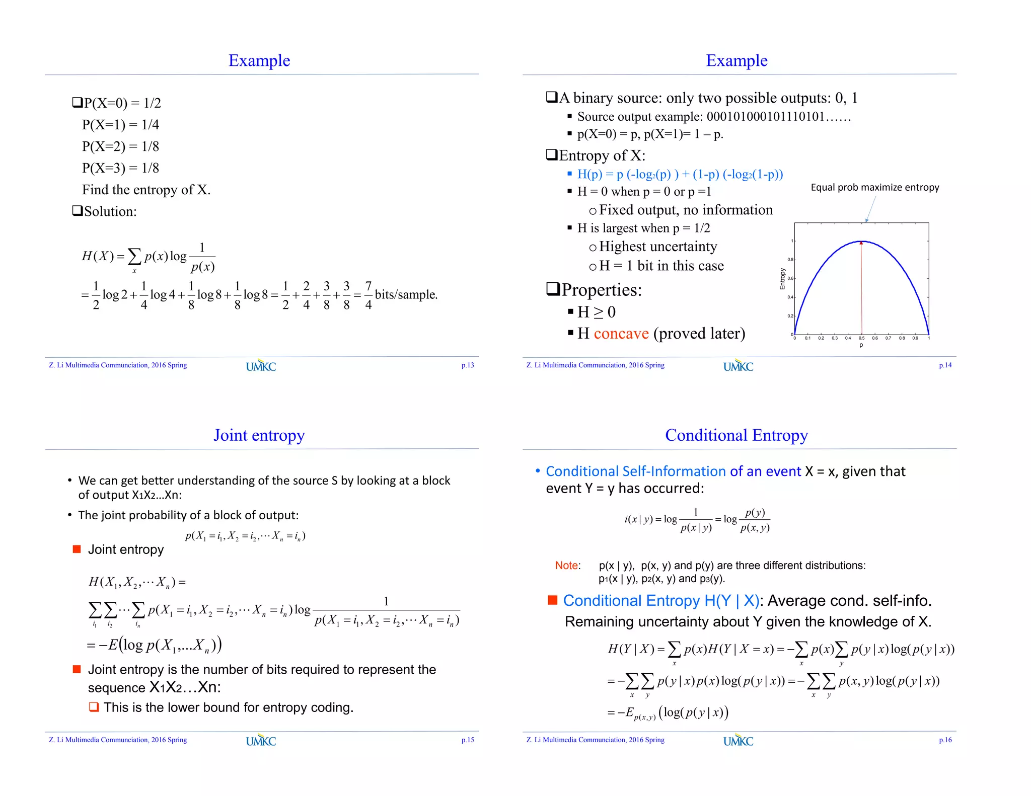
Conditional Entropy
Example: for the following joint distribution p(x, y), find H(Y |
X).
1 2 3 4
1 1/8 1/16 1/32 1/32
2 1/16 1/8 1/32 1/32
3 1/16 1/16 1/16 1/16
4 1/4 0 0 0
Y
X
( | ) ( ) ( | )log( ( | )) ( , )log( ( | ))
x y x y
H Y X p x p y x p y x p x y p y x     
Need to find conditional prob p(y | x)
( , )
( | )
( )
p x y
p y x
p x
 Need to find marginal prob p(x) first (sum columns).
P(X): [ ½, ¼, 1/8, 1/8 ] >> H(X) = 7/4 bits
P(Y): [ ¼ , ¼, ¼, ¼ ] >> H(Y) = 2 bits
H(X|Y) = ∑ = ( | = )
= ¼ H(1/2 ¼ 1/8 1/8 )
+ 1/4H(1/4, ½, 1/8 ,1/8)
+ 1/4H(1/4 ¼ ¼ ¼ ) +
1/4H(1 0 0 0)
= 11/8 bits
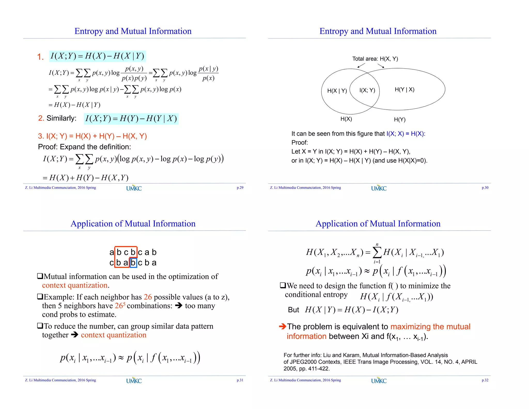
Chain Rule
H(X, Y) = H(X) + H(Y|X) = H(Y) + H(X|Y)
Proof:
H(X) H(Y)
H(X | Y) H(Y | X)
Total area: H(X, Y)
 








x
x yx y
x y
x y
XYHXHXYHxpxp
xypyxpxpyxp
xypxpyxp
yxpyxpYXH
).|()()|()(log)(
)|(log),()(log),(
)|()(log),(
),(log),(),(
Simpler notation:
)|()(
))|(log)((log)),((log),(
XYHXH
XYpXpEYXpEYXH


Conditional Entropy
Example: for the following joint distribution p(x, y), find H(Y |
X).
 Indeed, H(X|Y) = H(X, Y) – H(Y)= 27/8 – 2 = 11/8 bits
1 2 3 4
1 1/8 1/16 1/32 1/32
2 1/16 1/8 1/32 1/32
3 1/16 1/16 1/16 1/16
4 1/4 0 0 0
Y
X
P(X): [ ½, ¼, 1/8, 1/8 ] >> H(X) = 7/4 bits
P(Y): [ ¼ , ¼, ¼, ¼ ] >> H(Y) = 2 bits
H(X|Y) = ∑ = ( | = )
= ¼ H(1/2 ¼ 1/8 1/8 )
+ 1/4H(1/4, ½, 1/8 ,1/8)
+ 1/4H(1/4 ¼ ¼ ¼ ) +
1/4H(1 0 0 0)
= 11/8 bits
Chain Rule
 H(X,Y) = H(X) + H(Y|X)
 Corollary: H(X, Y | Z) = H(X | Z) + H(Y | X, Z)
Note that: ( , | ) ( | , ) ( | )p x y z p y x z p x z
(Multiply by p(z) at both sides, we get )( , , ) ( | , ) ( , )p x y z p y x z p x z
))|,((log)|,(log),,(
)|,(log)|,()()|,(
ZYXpEzyxpzyxp
zyxpzyxpzpZYXH
x y z
x yz




Proof:
),|()|(
)),|((log))|((log)|,(
ZXYHZXH
ZXYpEZXpEZYXH



General Chain Rule
General form of chain rule:
)...|(),...,( 1,1
1
21 XXXHXXXH i
n
i
in 


 The joint encoding of a sequence can be broken into the
sequential encoding of each sample, e.g.
H(X1, X2, X3)=H(X1) + H(X2|X1) + H(X3|X2, X1)
 Advantages:
 Joint encoding needs joint probability: difficult
 Sequential encoding only needs conditional entropy,
can use local neighbors to approximate the conditional entropy
 context-adaptive arithmetic coding.
Adding H(Z):  H(X, Y | Z) + H(z) = H(X, Y, Z)
= H(z) + H(X | Z) + H(Y | X, Z)
General Chain Rule
),...|()...|()(),...( 111211  nnn xxxpxxpxpxxpProof:
.),...|(
),...|(log),...(
),...|(log),...(
),...|(log),...(
),...(log),...(),...(
1
11
1 ,...1
111
,...1
11
1
1
,...1 1
111
,...1
111

 
 
 














n
i
ii
n
i xnx
iin
xnx
ii
n
i
n
xnx
n
i
iin
xnx
nnn
XXXH
xxxpxxp
xxxpxxp
xxxpxxp
xxpxxpXXH
General Chain Rule
1 1( | ,... )i ip x x x 
The complexity of the conditional probability
grows as the increase of i.
In many cases we can approximate the cond.
probability with some nearest neighbors (contexts):
1 1 1( | ,... ) ( | ,... )i i i i L ip x x x p x x x  
 The low-dim cond prob is more manageable
 How to measure the quality of the approximation?
 Relative entropy
0 1 1 0 1 0 1
a b c b c a b
c b a b c b a
Relative Entropy – Cost of Coding with Wrong Distr
Also known as Kullback Leibler (K-L) Distance, Information
Divergence, Information Gain
A measure of the “distance” between two distributions:
 In many applications, the true distribution p(X) is unknown, and we
only know an estimation distribution q(X)
 What is the inefficiency in representing X?
o The true entropy:
o The actual rate:
o The difference:






  )(
)(
log
)(
)(
log)()||(
Xq
Xp
E
xq
xp
xpqpD p
x
1 ( )log ( )
x
R p x p x 
2 ( )log ( )
x
R p x q x 
2 1 ( || )R R D p q 

Relative Entropy
Properties:






  )(
)(
log
)(
)(
log)()||(
Xq
Xp
E
xq
xp
xpqpD p
x
( || ) 0.D p q 
( || ) 0 if and only if q = p.D p q 
 What if p(x)>0, but q(x)=0 for some x?  D(p||q)=∞
 Caution: D(p||q) is not a true distance
 Not symmetric in general: D(p || q) ≠ D(q || p)
 Does not satisfy triangular inequality.
Proved later.
Relative Entropy
How to make it symmetric?
 Many possibilities, for example:
 
1
( || ) ( || )
2
D p q D q p
( || ) ( || )D p q D q p
 can be useful for pattern classification.
)||(
1
)||(
1
pqDqpD

Mutual Information
i (x | y): conditional self-information
)()(
),(
log
)(
)|(
log)|()();(
ypxp
yxp
xp
yxp
yxixiyxi 
Note: i(x; y) can be negative, if p(x | y) < p(x).
 Mutual information between two events:
i(x | y) = -log p(x | y)
 A measure of the amount of information that one
event contains about another one.
 or the reduction in the uncertainty of one event
due to the knowledge of the other.
Mutual Information
I(X; Y): Mutual information between two random variables:
  ( , )
( , )
( ; ) ( , ) ( ; ) ( , )log
( ) ( )
( , )
D ( , ) || ( ) ( ) log
( ) ( )
x y x y
p x y
p x y
I X Y p x y i x y p x y
p x p y
p X Y
p x y p x p y E
p X p Y
 
 
   
 
 
But it is symmetric: I(X; Y) = I(Y; X)
 Mutual information is a relative entropy:
 If X, Y are independent: p(x, y) = p(x) p(y)
 I (X; Y) = 0
 Knowing X does not reduce the uncertainty of Y.
Different from i(x; y), I(X; Y) >=0 (due to averaging)

Entropy and Mutual Information
( , ) ( | )
( ; ) ( , )log ( , )log
( ) ( ) ( )
( , )log ( | ) ( , )log ( )
( ) ( | )
x y x y
x y x y
p x y p x y
I X Y p x y p x y
p x p y p x
p x y p x y p x y p x
H X H X Y
 
 
 
 
 
2. Similarly: ( ; ) ( ) ( | )I X Y H Y H Y X 
1.
3. I(X; Y) = H(X) + H(Y) – H(X, Y)
Proof: Expand the definition:
( ; ) ( ) ( | )I X Y H X H X Y 
 
),()()(
)(log)(log),(log),();(
YXHYHXH
ypxpyxpyxpYXI
x y

 
Entropy and Mutual Information
H(X) H(Y)
I(X; Y)H(X | Y) H(Y | X)
Total area: H(X, Y)
It can be seen from this figure that I(X; X) = H(X):
Proof:
Let X = Y in I(X; Y) = H(X) + H(Y) – H(X, Y),
or in I(X; Y) = H(X) – H(X | Y) (and use H(X|X)=0).
Application of Mutual Information
a b c b c a b
c b a b c b a
Mutual information can be used in the optimization of
context quantization.
Example: If each neighbor has 26 possible values (a to z),
then 5 neighbors have 265 combinations:  too many
cond probs to estimate.
To reduce the number, can group similar data pattern
together  context quantization
  1 1 1 1( | ,... ) | ,...i i i ip x x x p x f x x 
Application of Mutual Information
We need to design the function f( ) to minimize the
conditional entropy
  1 1 1 1( | ,... ) | ,...i i i ip x x x p x f x x 
)...|(),...,( 1,1
1
21 XXXHXXXH i
n
i
in 


( | ) ( ) ( ; )H X Y H X I X Y But
The problem is equivalent to maximizing the mutual
information between Xi and f(x1, … xi-1).
))...(|( 1,1 XXfXH ii 
For further info: Liu and Karam, Mutual Information-Based Analysis
of JPEG2000 Contexts, IEEE Trans Image Processing, VOL. 14, NO. 4, APRIL
2005, pp. 411-422.

Outline
 Entropy Coding
 Prefix Coding
 Kraft-McMillan Inequality
 Shannon Codes
Variable Length Coding
Design the mapping from source symbols to codewords
Lossless mapping
Different codewords may have different lengths
Goal: minimizing the average codeword length
The entropy is the lower bound.
Classes of Codes
Non-singular code: Different inputs are mapped to different
codewords (invertible).
Uniquely decodable code: any encoded string has only one possible
source string, but may need delay to decode.
Prefix-free code (or simply prefix, or instantaneous):
No codeword is a prefix of any other codeword.
 The focus of our studies.
 Questions:
o Characteristic?
o How to design?
o Is it optimal?
All codes
Non-singular codes
Uniquely decodable
codes
Prefix-free codes
Prefix Code
 Examples
X
Singular Non-singular,
But not uniquely
decodable
Uniquely
decodable, but not
prefix-free
Prefix-free
1 0 0 0 0
2 0 010 01 10
3 0 01 011 110
4 0 10 0111 111
Need punctuation ……01011…
Need to look at next
bit to decode previous code.

Carter-Gill’s Conjecture [1974]
Carter-Gill’s Conjecture [1974]
 Every uniquely decodable code can be replaced by a prefix-free code
with the same set of codeword compositions.
 So we only need to study prefix-free code.
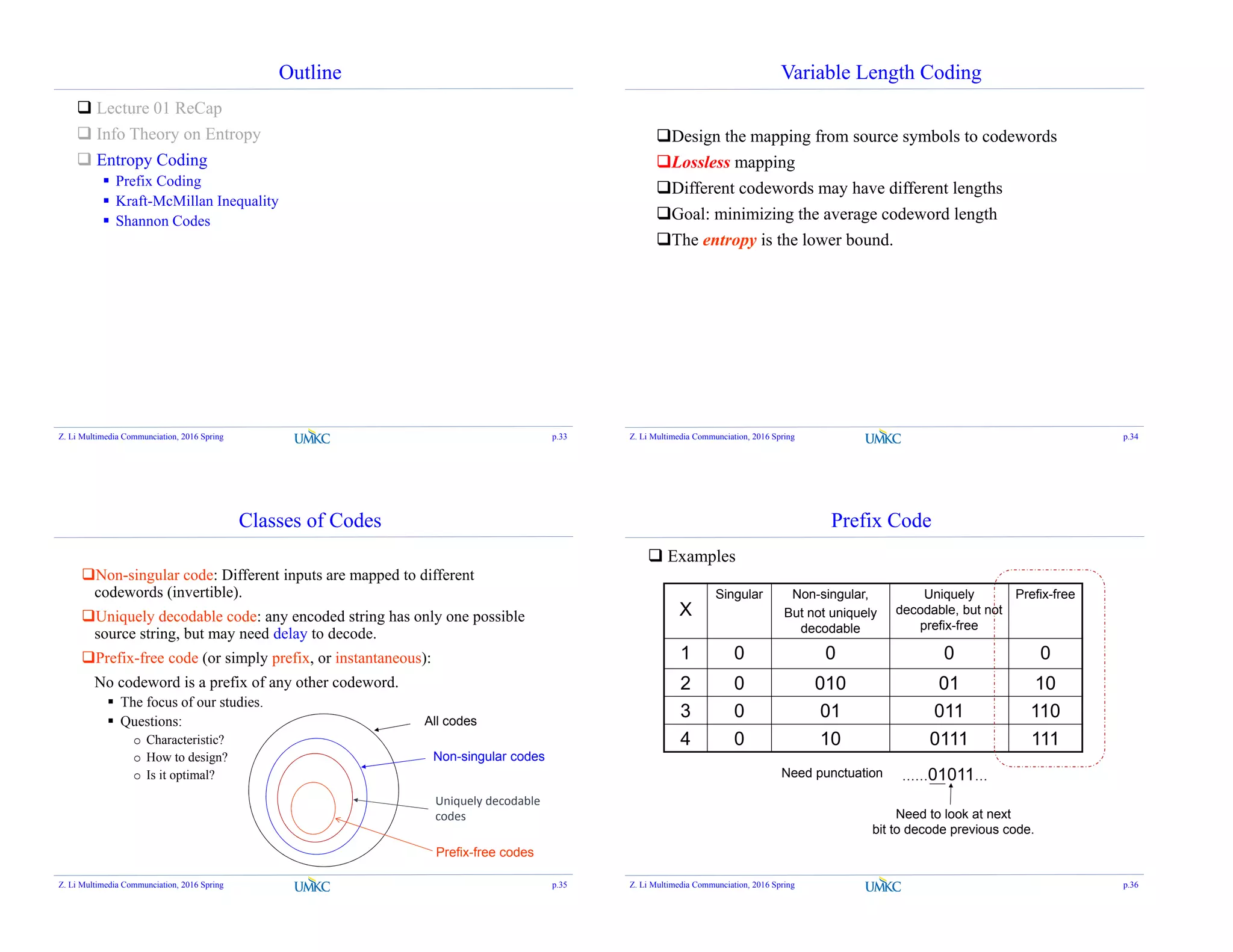
Prefix-free Code
Can be uniquely decoded.
No codeword is a prefix of another one.
Also called prefix code
Goal: construct prefix code with minimal expected length.
Can put all codewords in a binary tree:
0 1
0 1
0 1
0
10
110 111
Root node
leaf node
Internal node
 Prefix-free code contains leaves only.
 How to express the requirement mathematically?
Kraft-McMillan Inequality
12
1


N
i
li
• The codeword lengths li, i=1,…N of a prefix code over an
alphabet of size D(=2) satisfies the inequality
Conversely, if a set of {li} satisfies the inequality
above, then there exists a prefix code with codeword
lengths li, i=1,…N.
 The characteristic of prefix-free codes:
2212
11
L
N
i
lL
N
i
l ii
  



 Consider D=2: expand the binary code tree to full depth
L = max(li)
0
10
110
111
 Number of nodes in the last level:
 Each code corresponds to a sub-tree:
 The number of off springs in the last level:
 K-M inequality:
# of L-th level offsprings of all codes is less than 2^L !
ilL
2
L
2
L = 3
Example: {0, 10, 110, 111}
2^3=8
{4, 2, 0, 0}

0
10
110 111
11
Invalid code: {0, 10, 11, 110, 111}
Leads to more than
2^L offspring: 12> 23
12
1




i
li
 K-M inequality:
Extended Kraft Inequality
Countably infinite prefix code also satisfies the Kraft
inequality:
 Has infinite number of codewords.
Example:
 0, 10, 110, 1110, 11110, 111……10, ……
(Golomb-Rice code, next lecture)
 Each codeword can be mapped to a subinterval in [0, 1] that is
disjoint with others (revisited in arithmetic coding)
1
1




i
li
D
)
0
)
10
)
0 0.5 0.75 0.875 1
110 ……
0
10
110
….
L = 3
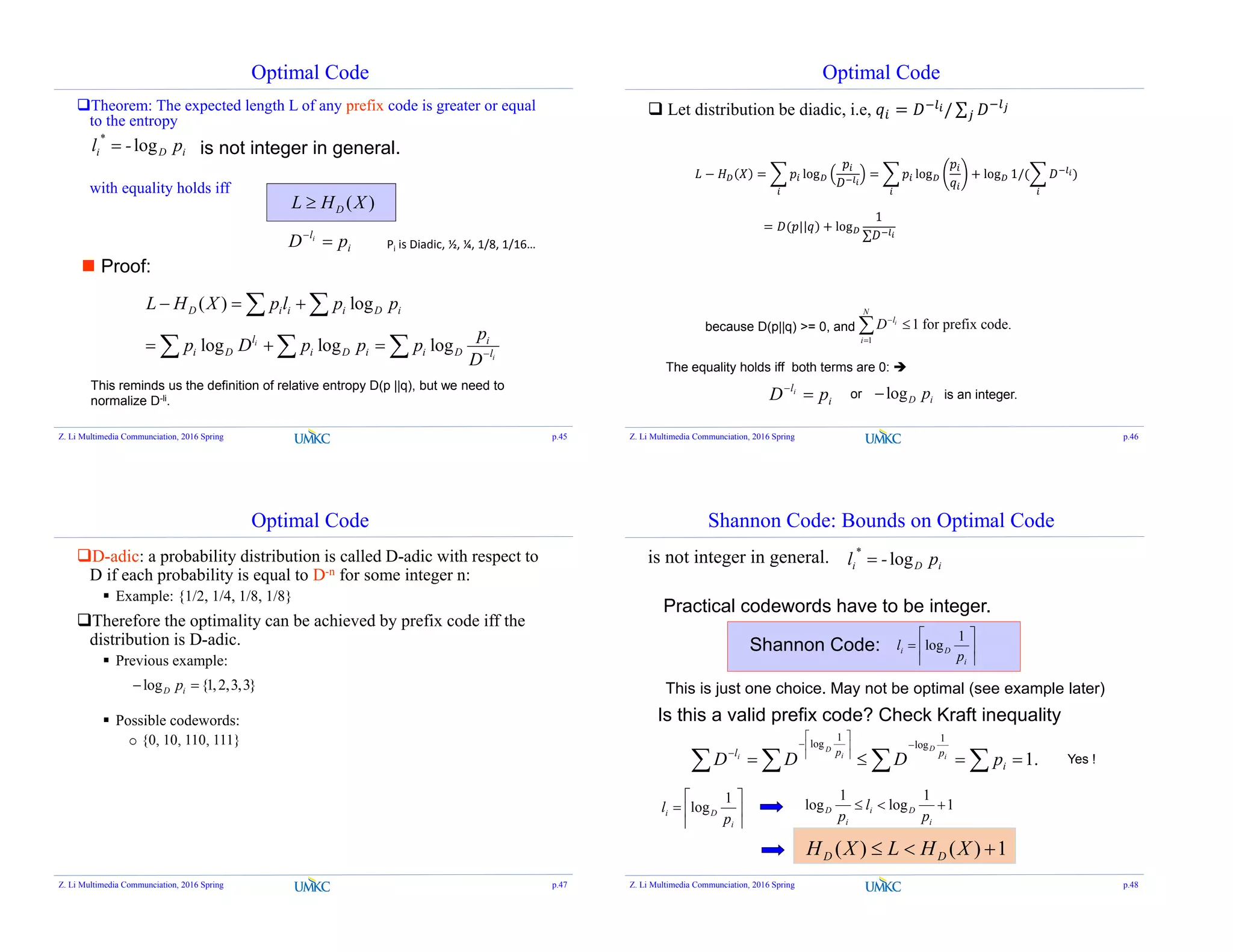
Optimal Codes (Advanced Topic)
How to design the prefix code with the minimal expected
length?
Optimization Problem: find {li} to
1..
min


 i
i
l
ii
l
Dts
lp
 Lagrangian solution:
 Ignore the integer codeword length constraint for now
 Assume equality holds in the Kraft inequality
 
 il
ii DlpJ Minimize
Optimal Codes
 
 il
ii DlpJ 
  0lnLet 

  il
i
i
DDp
l
J

 D
p
D ili
ln

1intongSubstituti   il
D
Dln
1

i
l
pD i

or
iDi pl log-
*

The optimal codeword length is the self-information of an event.
Expected codeword length:
)(log*
XHpplpL DiDiii    Entropy of X !

Optimal Code
Theorem: The expected length L of any prefix code is greater or equal
to the entropy
with equality holds iff
is not integer in general.iDi p-l log
*

( )DL H X
 Proof:
( ) log
log log logi
i
D i i i D i
l i
i D i D i i D l
L H X p l p p
p
p D p p p
D
  
  
 
  
This reminds us the definition of relative entropy D(p ||q), but we need to
normalize D-li.
i
l
pD i

Pi is Diadic, ½, ¼, 1/8, 1/16…
Optimal Code
 Let distribution be diadic, i.e, = / ∑
because D(p||q) >= 0, and
1
1 for prefix code.i
N
l
i
D


The equality holds iff both terms are 0: 
i
l
pD i

or logD ip is an integer.
− = log = log + log 1/( )
= ( | + log
1
∑
Optimal Code
D-adic: a probability distribution is called D-adic with respect to
D if each probability is equal to D-n for some integer n:
 Example: {1/2, 1/4, 1/8, 1/8}
Therefore the optimality can be achieved by prefix code iff the
distribution is D-adic.
 Previous example:
 Possible codewords:
o {0, 10, 110, 111}
log {1,2,3,3}D ip 
Shannon Code: Bounds on Optimal Code
is not integer in general. iDi p-l log
*

Practical codewords have to be integer.







i
Di
p
l
1
logShannon Code:
Is this a valid prefix code? Check Kraft inequality
.1
1
log
1
log
 








i
ppl
pDDD i
D
i
D
i
1
1
log
1
log 
i
Di
i
D
p
l
p






i
Di
p
l
1
log
1)()(  XHLXH DD
Yes !
This is just one choice. May not be optimal (see example later)

Optimal Code
The optimal code with integer lengths should be better than
Shannon code
1)()( *
 XHLXH DD
 To reduce the overhead per symbol:
 Encode a block of symbols {x1, x2, …, xn} together
 ),...,,(
1
),...,,(),...,,(
1
212121 nnnn xxxlE
n
xxxlxxxp
n
L  
  1),...,,(),...,,(),...,,( 212121  nnn XXXHxxxlEXXXH
Assume i.i.d. samples: )(),...,,( 21 XnHXXXH n 
n
XHLXH n
1
)()(  )(XHLn  if stationary.
(entropy rate)
Optimal Code
Impact of wrong pdf: what’s the penalty if the pdf we use is different
from the true pdf?
True pdf: p(x) Codeword length: l(x)
Estimated pdf: q(x) Expected length: Epl(X)
1)||()()()||()(  qpDpHXlEqpDpH p
Proof: assume Shannon code 






)(
1
log)(
xq
xl
 











 1
)(
1
log)(
)(
1
log)()(
xq
xp
xq
xpXlEp
1)||()(1
)(
1
)(
)(
log)( 













  qpDXH
xpxq
xp
xp
The lower bound is derived similarly.
Shannon Code is not optimal
Example:
 Binary r.v. X: p(0)=0.9999, p(1)=0.0001.
Entropy: 0.0015 bits/sample
Assign binary codewords by Shannon code:







)(
1
log)(
xp
xl
.1
9999.0
1
log2 



.14
0001.0
1
log2 





 Expected length: 0.9999 x 1+ 0.0001 x 14 = 1.0013.
 Within the range of [H(X), H(X) + 1].
 But we can easily beat this by the code {0, 1}
 Expected length: 1.
Q&A

Multimedia Communication Lec02: Info Theory and Entropy

More Related Content

What's hot

Viewers also liked

Similar to Multimedia Communication Lec02: Info Theory and Entropy

More from United States Air Force Academy

Recently uploaded

Multimedia Communication Lec02: Info Theory and Entropy