Download as PDF, PPTX

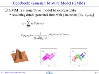
![VL_FEAT: vl_dsift
Compute dense SIFT as a texture descriptor for the
image
[f, dsift]=vl_dsift(single(rgb2gray(im)), ‘step’, 2);
There’s also a FAST option
[f, dsift]=vl_dsift(single(rgb2gray(im)), ‘fast’, ‘step’, 2);
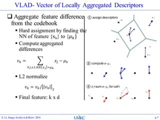
Huge amount of SIFT data will be generated
Z. Li, Image Analysis&Retrv.2016 p.11](https://image.slidesharecdn.com/lec08-161108175346/85/Lec-08-Feature-Aggregation-II-Fisher-Vector-AKULA-and-Super-Vector-11-320.jpg)
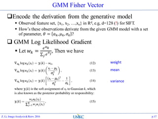
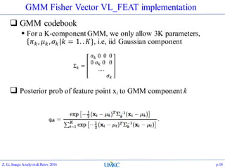
![GMM Fisher Vector VL_FEAT implementation
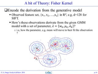
FV encoding
Gradient on the mean, for GMM component k, j=1..D
In the end, we have 2K x D aggregation on the derivation
w.r.t. the means and variances
Z. Li, Image Analysis&Retrv.2016 p.19
𝐹𝑉 = [𝑢1, 𝑢2,… , 𝑢 𝐾, 𝑣1, 𝑣2, … , 𝑣 𝐾]](https://image.slidesharecdn.com/lec08-161108175346/85/Lec-08-Feature-Aggregation-II-Fisher-Vector-AKULA-and-Super-Vector-19-320.jpg)
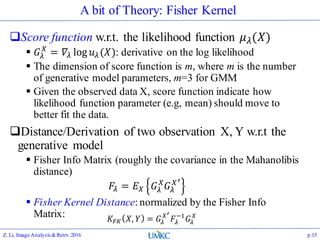
![VL_FEAT GMM/FV API
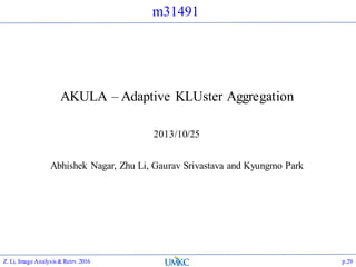
Compute GMM model with VL_FEAT
Prepare data:
numPoints = 1000 ; dimension = 2 ;
data = rand(dimension,N) ;
Call vl_gmm:
numClusters = 30 ;
[means, covariances, priors] = vl_gmm(data, numClusters) ;
Visualize:
figure ;
hold on ;
plot(data(1,:),data(2,:),'r.') ;
for i=1:numClusters
vl_plotframe([means(:,i)' sigmas(1,i) 0 sigmas(2,i)]);
end
Z. Li, Image Analysis&Retrv.2016 p.20](https://image.slidesharecdn.com/lec08-161108175346/85/Lec-08-Feature-Aggregation-II-Fisher-Vector-AKULA-and-Super-Vector-20-320.jpg)
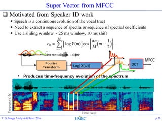
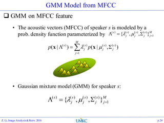
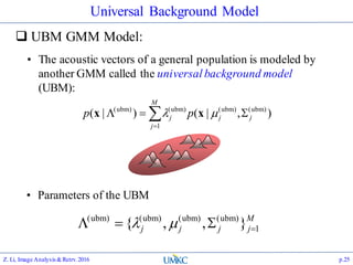
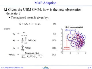
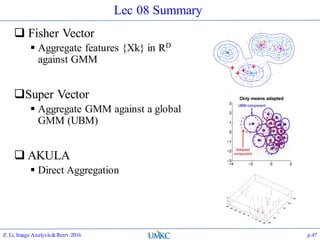

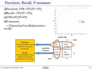
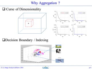
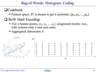
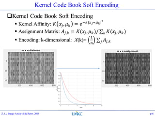
The document outlines the content of a lecture series on image analysis and retrieval focusing on feature aggregation techniques such as Fisher vectors, VLAD, and Akula. It discusses the significance of precision, recall, and various coding schemes including bag-of-words and Gaussian mixture models. Additionally, it covers methods for aggregating features for applications like speaker identification, providing a detailed explanation of their implementation and theoretical underpinnings.


![OpenGL Mini Projects With Source Code [ Computer Graphics ]](https://cdn.slidesharecdn.com/ss_thumbnails/newmicrosoftpowerpointpresentation-180330204024-thumbnail.jpg?width=640&height=640&fit=bounds)