Lec-03 Entropy Coding I: Hoffmann & Golomb Codes

CS/EE 5590 / ENG 401 Special Topics
(Class Ids: 17804, 17815, 17803)
Lec 03
Entropy and Coding II
Hoffman and Golomb Coding
Zhu Li
Z. Li Multimedia Communciation, 2016 Spring p.1
Outline
 Lecture 02 ReCap
 Hoffman Coding
 Golomb Coding and JPEG 2000 Lossless Coding
Entropy
 Self Info of an event
= = − log Pr = =
− log ( )
 Entropy of a source
= ∑ log ( )
Conditional Entropy, Mutual Information
= , − ( )
, = + − ,
H(X) H(Y)
I(X; Y)H(X | Y) H(Y | X)
Total area: H(X, Y)
a b c b c a b
c b a b c b a
Main application: Context
Modeling
Relative Entropy
( | = log

Context Reduces Entropy Example
x1 x2 x3
x4 x5
H(x5) > H(x5|x4,x3, x2,x1)
H(x5) > H(x5|f(x4,x3, x2,x1))
Condition reduces entropy:
Context function:
f(x4,x3, x2,x1)= sum(x4,x3, x2,x1)
getEntropy.m, lossless_coding.m
f(x4,x3, x2,x1)==100
f(x4,x3, x2,x1)<100
Context:

Lossless Coding
 Prefix Coding
 Codes on leaves
 No code is prefix of other codes
 Simple encoding/decoding
Kraft- McMillan Inequality:
 For a coding scheme with code length: l1, l2, …ln,
 Given a set of integer length {l1, l2, …ln} that satisfy above inequality,
we can always find a prefix code with code length l1, l2, …ln
0 1
0 1
0 1
0
10
110 111
Root node
leaf node
Internal node
2 ≤ 1
Outline
 Hoffman Coding
 Golomb Coding and JPEG 2000 Lossless
Huffman Coding
A procedure to construct optimal prefix code
Result of David Huffman’s term paper in 1952 when he was a
PhD student at MIT
 Shannon  Fano  Huffman (1925-1999)
Huffman Code Design
 Requirement:
 The source probability distribution.
(But not available in many cases)
 Procedure:
1. Sort the probability of all source symbols in a descending order.
2. Merge the last two into a new symbol, add their probabilities.
3. Repeat Step 1, 2 until only one symbol (the root) is left.
4. Code assignment:
Traverse the tree from the root to each leaf node,
assign 0 to the top branch and 1 to the bottom branch.

Example
Source alphabet A = {a1, a2, a3, a4, a5}
Probability distribution: {0.2, 0.4, 0.2, 0.1, 0.1}
a2 (0.4)
a1(0.2)
a3(0.2)
a4(0.1)
a5(0.1)
Sort
0.2
merge Sort
0.4
0.2
0.2
0.2
0.4
merge Sort
0.4
0.2
0.4
0.6
merge
0.6
0.4
Sort
1
merge
Assign code
0
1
1
00
01
1
000
001
01
1
000
01
0010
0011
1
000
01
0010
0011
Huffman code is prefix-free
01 (a1)
000 (a3)
0010 (a4) 0011(a5)
1
000
01
0010
0011
1 (a2)
All codewords are leaf nodes
 No code is a prefix of any other code.
(Prefix free)
Average Codeword Length vs Entropy
 Source alphabet A = {a, b, c, d, e}
 Probability distribution: {0.2, 0.4, 0.2, 0.1, 0.1}
 Code: {01, 1, 000, 0010, 0011}
 Entropy:
H(S) = - (0.2*log2(0.2)*2 + 0.4*log2(0.4)+0.1*log2(0.1)*2)
= 2.122 bits / symbol
 Average Huffman codeword length:
L = 0.2*2+0.4*1+0.2*3+0.1*4+0.1*4 = 2.2 bits / symbol
 This verifies H(S) ≤ L < H(S) + 1.
Huffman Code is not unique
0.4
0.2
0.4
0.6
0.6
0.4
0
1
1
00
01
 Multiple ordering choices for tied probabilities
 Two choices for each split: 0, 1 or 1, 0
0.4
0.2
0.4
0.6
0.6
0.4
1
0
0
10
11
a
b
c
0.4
0.2
0.4
0.6
0.6
0.4
1
0
0
10
11
b
a
c
0.4
0.2
0.4
0.6
0.6
0.4
1
0
0
10
11

Huffman Coding is Optimal
Assume the probabilities are ordered:
 p1 ≥ p2 ≥ …… pm.
Lemma: For any distribution, there exists an optimal
prefix code that satisfies:
 If pj ≥ pk, then lj ≤ lk: otherwise can swap codewords to reduce
the average length.
The two least probable letters have the same length:
otherwise we can truncate the longer one without violating
prefix-free condition.
The two longest codewords differ only in the last bit and
correspond to the two least probable symbols. Otherwise we
can rearrange to achieve this.
 Proof skipped.
Canonical Huffman Code
 Huffman algorithm is needed only to compute the optimal
codeword lengths
 The optimal codewords for a given data set are not unique
 Canonical Huffman code is well structured
 Given the codeword lengths, can find a canonical Huffman
code
 Also known as slice code, alphabetic code.
Canonical Huffman Code
Example:
 Codeword lengths: 2, 2, 3, 3, 3, 4, 4
 Verify that it satisfies Kraft-McMillan inequality
01
100
11
000 001
1010 1011
A non-canonical example
00 01
The Canonical Tree
 Rules:
 Assign 0 to left branch and 1 to right branch
 Build the tree from left to right in increasing order of depth
 Each leaf is placed at the first available position
110100 101
10
1110 1111
111
12
1


N
i
li
Canonical Huffman
Properties:
 The first code is a series of 0
 Codes of same length
are consecutive: 100, 101, 110
 If we pad zeros to the right side such that all
codewords have the same length, shorter codes would
have lower value than longer codes:
0000 < 0100 < 1000 < 1010 < 1100 < 1110 < 1111
00 01
110100 101
1110 1111
 If from length n to n + 2 directly:
e.g., 1, 3, 3, 3, 4, 4
C(n+2, 1) = 4( C(n, last) + 1)
0
110100 101
1110 1111
First code
of length n+1
Last code of
length n
 Coding from length level n to level n+1:
 C(n+1, 1) = 2 ( C(n, last) + 1): append a 0 to the next available level-n code

Advantages of Canonical Huffman
1. Reducing memory requirement
 Non-canonical tree needs:
All codewords
Lengths of all codewords
 Need a lot of space for large table
01
100
11
000 001
1010 1011
00 01
110100 101
1110 1111
 Canonical tree only needs:
 Min: shortest codeword length
 Max: longest codeword length
 Distribution:
 Number of codewords in each level
 Min=2, Max=4,
# in each level: 2, 3, 2
Outline
 Hoffman Coding
 Golomb Coding
Unary Code (Comma Code)
Encode a nonnegative integer n by n 1’s and a 0
(or n 0’s and an 1).
n Codeword
0 0
1 10
2 110
3 1110
4 11110
5 111110
… …
 Is this code prefix-free?
0 1
0 1
0 1
0
10
110
1110
… …
 When is this code optimal?
 When probabilities are: 1/2, 1/4, 1/8, 1/16, 1/32 …  D-adic
 Huffman code becomes unary code in this case.
 No need to store codeword table, very simple
Implementation – Very Efficient
Encoding:
UnaryEncode(n) {
while (n > 0) {
WriteBit(1);
n--;
}
WriteBit(0);
}
 Decoding:
UnaryDecode() {
n = 0;
while (ReadBit(1) == 1) {
n++;
}
return n;
}

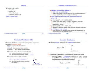
Golomb Code [Golomb, 1966]
A multi-resolutional approach:
 Divide all numbers into groups of equal size m
o Denote as Golomb(m) or Golomb-m
 Groups with smaller symbol values have shorter codes
 Symbols in the same group has codewords of similar lengths
o The codeword length grows much slower than in unary code
0 max
m m m m
 Codeword :
 (Unary, fixed-length)
Group ID:
Unary code
Index within each group:
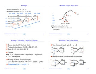
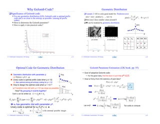
Golomb Code
rm
m
n
rqmn 




 q: Quotient,
used unary code
q Codeword
0 0
1 10
2 110
3 1110
4 11110
5 111110
6 1111110
… …
 r: remainder, “fixed-length” code
 K bits if m = 2^k
 m=8: 000, 001, ……, 111
 If m ≠ 2^k: (not desired)
bits for smaller r
bits for larger r
 m2log
 m2log
m = 5: 00, 01, 10, 110, 111
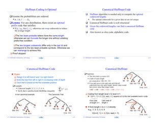
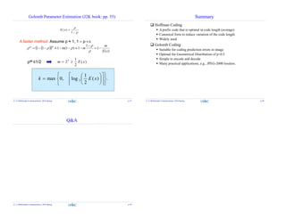
Golomb Code with m = 5 (Golomb-5)
n q r code
0 0 0 000
1 0 1 001
2 0 2 010
3 0 3 0110
4 0 4 0111
n q r code
5 1 0 1000
6 1 1 1001
7 1 2 1010
8 1 3 10110
9 1 4 10111
n q r code
10 2 0 11000
11 2 1 11001
12 2 2 11010
13 2 3 110110
14 2 4 110111
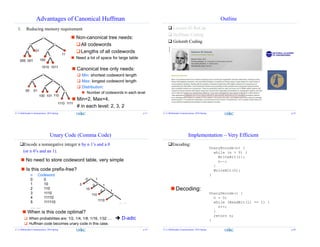
Golomb vs Canonical Huffman
Golomb code is a canonical Huffman
 With more properties
 Codewords: 000, 001, 010, 0110, 0111,
1000, 1001, 1010, 10110, 10111
 Canonical form:
From left to right
From short to long
Take first valid spot

 A special Golomb code with m= 2^k
 The remainder r is the fixed k LSB bits of n
n q r code
0 0 0 0000
1 0 1 0001
2 0 2 0010
3 0 3 0011
4 0 4 0100
5 0 5 0101
6 0 6 0110
7 0 7 0111
n q r code
8 1 0 10000
9 1 1 10001
10 1 2 10010
11 1 3 10011
12 1 4 10100
13 1 5 10101
14 1 6 10110
15 1 7 10111
 m = 8
Golobm-Rice Code
Implementation
Encoding:
GolombEncode(n, RBits) {
q = n >> RBits;
UnaryCode(q);
WriteBits(n, RBits);
}
 Decoding:
GolombDecode(RBits) {
q = UnaryDecode();
n = (q << RBits) + ReadBits(RBits);
return n;
}
Remainder bits:
RBits = 3 for m = 8
Output the lower (RBits) bits of n.
n q r code
0 0 0 0000
1 0 1 0001
2 0 2 0010
3 0 3 0011
4 0 4 0100
5 0 5 0101
6 0 6 0110
7 0 7 0111
Exponential Golomb Code (Exp-Golomb)
Golomb code divides the alphabet into
groups of equal size
0 max
m m m m
 In Exp-Golomb code, the group size
increases exponentially
 Codes still contain two parts:
 Unary code followed by fixed-length code
0 max
4 8 161 2
n code
0 0
1 100
2 101
3 11000
4 11001
5 11010
6 11011
7 1110000
8 1110001
9 1110010
10 1110011
11 1110100
12 1110101
13 1110110
14 1110111
15 111100000
 Proposed by Teuhola in 1978
Implementation
Decoding
ExpGolombDecode() {
GroupID = UnaryDecode();
if (GroupID == 0) {
return 0;
} else {
Base = (1 << GroupID) - 1;
Index = ReadBits(GroupID);
return (Base + Index);
}
}
}
n code Group
ID
0 0 0
1 100 1
2 101
3 11000 2
4 11001
5 11010
6 11011
7 1110000 3
8 1110001
9 1110010
10 1110011
11 1110100
12 1110101
13 1110110
14 1110111

Outline
Golomb Code Family:
 Unary Code
 Golomb Code
 Golomb-Rice Code
 Exponential Golomb Code
Why Golomb code?
Geometric Distribution (GD)
 Geometric distribution with parameter ρ:
 P(x) = ρx (1 - ρ), x ≥ 0, integer.
 Prob of the number of failures before the first success in a series of
independent Yes/No experiments (Bernoulli trials).
 Unary code is the optimal prefix code for geometric distribution
with ρ ≤ 1/2:
 ρ = 1/4: P(x): 0.75, 0.19, 0.05, 0.01, 0.003, …
 Huffman coding never needs to re-order  equivalent to unary code.
 Unary code is the optimal prefix code, but not efficient
( avg length >> entropy)
 ρ = 3/4: P(x): 0.25, 0.19, 0.14, 0.11, 0.08, …
 Reordering is needed for Huffman code, unary code not optimal prefix code.
 ρ = 1/2: Expected length = entropy.
 Unary code is not only the optimal prefix code, but also optimal among all
entropy coding (including arithmetic coding).
Geometric Distribution (GD)
Geometric distribution is very useful for image/video compression
Example 1: run-length coding
 Binary sequence with i.i.d. distribution
 P(0) = ρ ≈ 1:
 Example: 0000010000000010000110000001
 Entropy << 1, prefix code has poor performance.
 Run-length coding is efficient to compress the data:
or: Number of consecutive 0’s between two 1’s
o  run-length representation of the sequence: 5, 8, 4, 0, 6
 Probability distribution of the run-length r:
o P(r = n) = ρn (1- ρ): n 0’s followed by an 1.
o  The run has one-sided geometric distribution
with parameter ρ.
r
P(r)
Geometric Distribution
GD is the discrete analogy of the Exponential distribution
x
exf

 
)( 2
1
Two-sided geometric distribution is the discrete
analogy of the Laplacian distribution (also called
double exponential distribution)
( ) x
f x e 
 

x
f(x)
x
f(x)

Why Golomb Code?
Significance of Golomb code:
 For any geometric distribution (GD), Golomb code is optimal prefix
code and is as close to the entropy as possible (among all prefix
codes)
 How to determine the Golomb parameter?
 How to apply it into practical codec?
Geometric Distribution
Example 2: GD is a also good model for Prediction error
e(n) = x(n) – pred(x(1), …, x(n-1)).
Most e(n)’s have smaller values around 0:
 can be modeled by geometric distribution.
n
p(n)
10,
1
1
)( ||



 

 n
np
x1 x2 x3
x4 x5
0.2 0.3 0.2
0.2 0 0
0 0 0
Optimal Code for Geometric Distribution
 Geometric distribution with parameter ρ:
 P(X=n) = ρn (1 - ρ)
 Unary code is optimal prefix code when ρ ≤ 1/2.
 Also optimal among all entropy coding for ρ = 1/2.
 How to design the optimal code when ρ > 1/2 ?
x
P(x)
1 1
0 0
1
( ) ( ) (1 ) (1 ) (1 )
1q
mm m
qm r qm mq m
X X
r r
P q P qm r

     

 

 

       

 
 xq has geometric dist with parameter ρm.
Unary code is optimal for xq if ρm ≤ 1/2 
2log
1
m integer.possibleminimaltheis
log
1
2








m
rq xmxx 
 Transform into GD with ρ ≤ 1/2 (as close as possible)
How? By grouping m events together!
Each x can be written as
x
P(x)
Golomb Parameter Estimation (J2K book: pp. 55)
x
xP )1()( 
• Goal of adaptive Golomb code:
• For the given data, find the best m such that ρm ≤1/2.
• How to find ρ from the statistics of past data?








 

 1)1(
)1()1()( 2
0x
x
xxE
.
)(1
)(
xE
xE


2
1
)(1
)(








m
m
xE
xE
 




 

)(
)(1
log/1
xE
xE
m
Let m=2k
.
)(
)(1
log/1log 22 












 

xE
xE
k Too costly to compute

Golomb Parameter Estimation (J2K book: pp. 55)
( )
1
E x




A faster method: Assume ρ ≈ 1, 1 – ρ ≈ 0.
  
)(
1
1
1)1(111
xE
m
mm
mm






ρm ≤1/2 )(
2
1
2 xEm k

.)(
2
1
log,0max 2


















 xEk
Summary
 Hoffman Coding
 A prefix code that is optimal in code length (average)
 Canonical form to reduce variation of the code length
 Widely used
 Golomb Coding
 Suitable for coding prediction errors in image
 Optimal for Geometrical Distribution of p=0.5
 Simple to encode and decode
 Many practical applications, e.g., JPEG-2000 lossless.
Q&A

Lec-03 Entropy Coding I: Hoffmann & Golomb Codes

More Related Content

What's hot

Viewers also liked

Similar to Lec-03 Entropy Coding I: Hoffmann & Golomb Codes

More from United States Air Force Academy

Recently uploaded

Lec-03 Entropy Coding I: Hoffmann & Golomb Codes