Download as PDF, PPTX
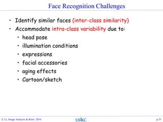
![SVD as Signal Decomposition
The Singular Value Decomposition (SVD) of an nxm matrix A,
is,
Where the diagonal of S are the eigen values of AAT,
[𝜎1, 𝜎2, … , 𝜎 𝑛], called “singular values”
U are eigenvectors of AAT, and V are eigen vectors of ATA,
the outer product of uivi
T, are basis of A in reconstruction:
𝐴 = 𝑈𝑆𝑉 𝑇 =
𝑖
𝜎𝑖 𝑢𝑖 𝑣𝑖
𝑡
A(mxn) = U(mxm) S(mxn)
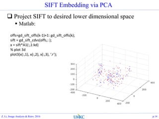
V(nxn)
The 1st order SVD approx. of A is:
𝜎1 ∗ 𝑈 : , 1 ∗ 𝑉 : , 1 𝑇
Z. Li, Image Analysis & Retrv. 2016 p.4](https://image.slidesharecdn.com/lec14-eigenfaceandfisherface-161108174733/85/Lec14-eigenface-and-fisherface-4-320.jpg)
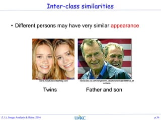
![SVD approximation of an image
Very easy…
function [x]=svd_approx(x0, k)
dbg=0;
if dbg
x0= fix(100*randn(4,6));
k=2;
end
[u, s, v]=svd(x0);
[m, n]=size(s);
x = zeros(m, n);
sgm = diag(s);
for j=1:k
x = x + sgm(j)*u(:,j)*v(:,j)';
end
Z. Li, Image Analysis & Retrv. 2016 p.5](https://image.slidesharecdn.com/lec14-eigenfaceandfisherface-161108174733/85/Lec14-eigenface-and-fisherface-5-320.jpg)
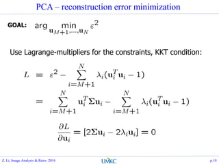
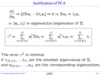
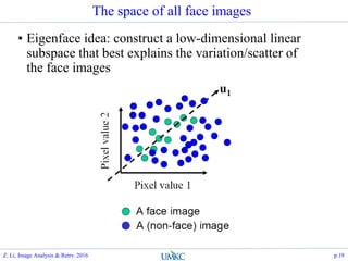
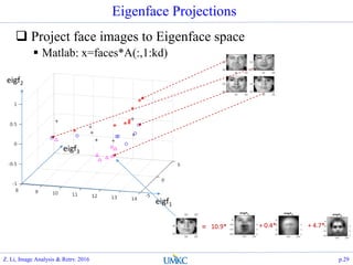
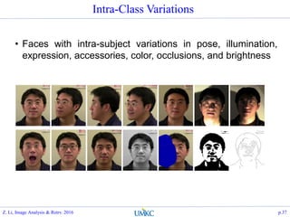
![PCA- Principal Component Analysis
Formulation:
Find projections, that the information/energy of the data are
maximally preserved
Matlab: [A, s, eigv]=princomp(X);
max
𝑊
𝐸 𝑥 𝑇 𝑊 𝑇 𝑊𝑥 , 𝑠. 𝑡. , 𝑊 𝑇 𝑊 = 𝐼
Z. Li, Image Analysis & Retrv. 2016 p.6](https://image.slidesharecdn.com/lec14-eigenfaceandfisherface-161108174733/85/Lec14-eigenface-and-fisherface-6-320.jpg)
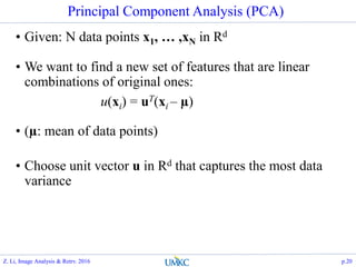
![PCAAlgorithm
Center the data:
X = X – repmat(mean(x), [n,
1]);
Principal component #1
points in the direction of the
largest variance
Each subsequent principal
component…
is orthogonal to the previous
ones, and
points in the directions of the
largest variance of the residual
subspace
Solved by finding Eigen
Vectors of the
Scatter/Covarinace matrix of
data:
S = cov(X); [A, eigv]=Eig(S)
Z. Li, Image Analysis & Retrv. 2016 p.7](https://image.slidesharecdn.com/lec14-eigenfaceandfisherface-161108174733/85/Lec14-eigenface-and-fisherface-7-320.jpg)

![Matlab Implementation
Scaling the face image to thumbnail size
Justification: as long as human eye can recognize, that
contains sufficient info
Scale space characteristic response for face recognition
Compute the PCA over the vectorized face data
load faces-ids-n6680-m417-20x20.mat;
[A, s, lat]=princomp(faces);
h=20; w=20;
figure(30);
subplot(1,2,1); grid on; hold on; stem(lat, '.');
f_eng=lat.*lat;
subplot(1,2,2); grid on; hold on; plot(cumsum(f_eng)/sum(f_eng),
'.-');
Z. Li, Image Analysis & Retrv. 2016 p.27](https://image.slidesharecdn.com/lec14-eigenfaceandfisherface-161108174733/85/Lec14-eigenface-and-fisherface-27-320.jpg)
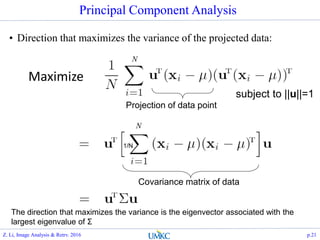
![Eigenface
Holistic approach: treat an hxw image as a point in Rhxw:
Face data set: 20x20 face icon images, 417 subjects, 6680 face images
Notice that all the face images are not filling up the R20x20 space:
Eigenface basis: imagesc(reshape(A1(:,1), [h, w]));
kd kd
eigval
Infopreservingratio
Z. Li, Image Analysis & Retrv. 2016 p.28](https://image.slidesharecdn.com/lec14-eigenfaceandfisherface-161108174733/85/Lec14-eigenface-and-fisherface-28-320.jpg)
![Eigenface Matlab
Matlab code
% PCA:
[A, s, eigv]=princomp(faces);
kd=16; nface=120;
% eigenface projectio
x=faces*A(:, 1:kd);
f_dist = pdist2(x(1:nface,:), x(1:nface,:));
figure(32);
imagesc(f_dist); colormap('gray');
figure(33); hold on; grid on;
d0 = f_dist(1:7,1:7); d1=f_dist(8:end, 8:end);
[tp, fp, tn, fn]= getPrecisionRecall(d0(:), d1(:), 40);
plot(fp./(tn+fp), tp./(tp+fn), '.-r', 'DisplayName', 'tpr-fpr
color, data set 1');
xlabel('fpr'); ylabel('tpr'); title('eig face recog');
legend('kd=8', 'kd=12', 'kd=16', 0);
Z. Li, Image Analysis & Retrv. 2016 p.31](https://image.slidesharecdn.com/lec14-eigenfaceandfisherface-161108174733/85/Lec14-eigenface-and-fisherface-31-320.jpg)


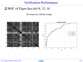
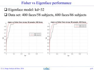
![Experiment results on 417-6680 data set
Compute Eigenface model and Fisherface model
% Eigenface: A1
load faces-ids-n6680-m417-20x20.mat;
[A1, s, lat]=princomp(faces);
% Fisherface: A2
n_face = 600; n_subj = length(unique(ids(1:n_face)));
%eigenface kd
kd = 32; opt.Fisherface = 1;
[A2, lat]=LDA(ids(1:n_face), opt,
faces(1:n_face,:)*A1(:,1:kd));
% eigenface
x1 = faces*A1(:,1:kd);
f_dist1 = pdist2(x1, x1);
% fisherface
x2 = faces*A1(:,1:kd)*A2;
f_dist2 = pdist2(x2, x2);
Z. Li, Image Analysis & Retrv. 2016 p.44](https://image.slidesharecdn.com/lec14-eigenfaceandfisherface-161108174733/85/Lec14-eigenface-and-fisherface-44-320.jpg)
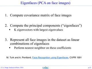
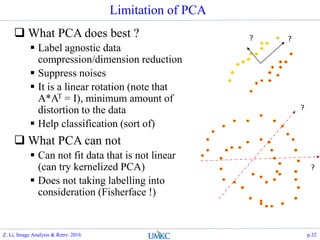
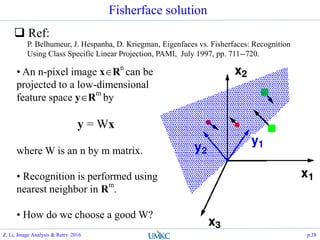
![Summary
PCA approach
Try to find an orthogonal rotation
s.t. the first k-dimensions of the
new subspace, captures most of
the info of the data
Agnostic to the label info
Matlab: [A, s,
eigv]=princomp(data);
LDA approach
Try to find projection that
maximizes the ratio of between
class scatter vs within class
scatter
Typically solved by apply PCA
first to avoid within class scatter
singularity
Utilizes label info
Matlab: [A, eigv]=LDA(label,
opt, data);
1
2
PCA
Fisher
Z. Li, Image Analysis & Retrv. 2016 p.46](https://image.slidesharecdn.com/lec14-eigenfaceandfisherface-161108174733/85/Lec14-eigenface-and-fisherface-46-320.jpg)

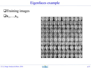
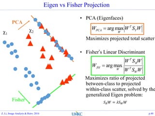
The document discusses image analysis and retrieval techniques, focusing on methods such as Singular Value Decomposition (SVD) and Principal Component Analysis (PCA) for face recognition tasks. It outlines the processes of eigenfaces and fisherfaces, emphasizing the importance of dimensionality reduction and how these methods can improve recognition accuracy by addressing the challenges posed by variability in facial characteristics. Further, it details the limitations of PCA and the rationale behind using Fisher's Linear Discriminant to enhance performance in classification tasks.