Download as PDF, PPTX
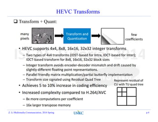


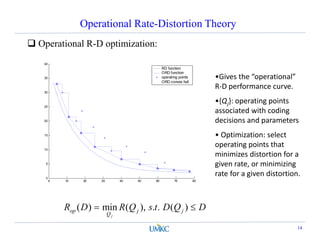
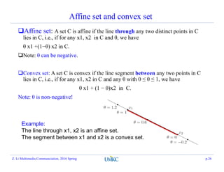
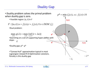
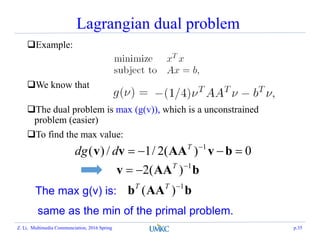
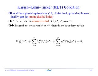
![Lower bound on optimal value
Solid line: f0(x)
Dashed line: f1(x)
Feasible set: [-0.46, 0.46] (f1(x) <=0)
Optimal solution: x* = -0.46, p* = 1.54
Dotted line: L(x, λ) for λ = 0.1, 0.2, …, 1.0.
The minimum of each dotted line is <= p*.
Dual function g(λ)= inf L(x, λ).
(Note that fi(x) is not convex,
But g(λ) is concave!)
Dashed line: p*.
.0)(..),(min 10 xftsxf
)(0 xf
)(1 xf
),( xL
Z. Li, Multimedia Communciation, 2016 Spring p.32](https://image.slidesharecdn.com/lec11-ratedistortionoptimization-160320211617/85/Lec11-rate-distortion-optimization-32-320.jpg)


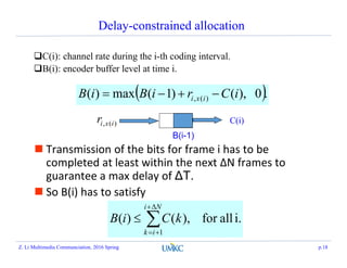
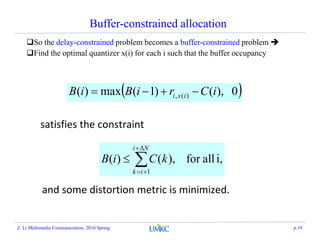
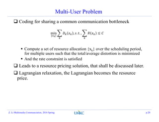
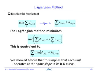
This document summarizes a lecture on rate-distortion optimization in video coding. It discusses various rate-distortion optimization problems including operational rate-distortion theory, joint source-channel coding optimization, storage constraint allocation, delay-constrained allocation, buffer-constrained allocation, and the multi-user problem. It also covers convex optimization techniques like the Lagrangian method that can help solve some of these optimization problems.