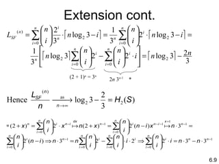
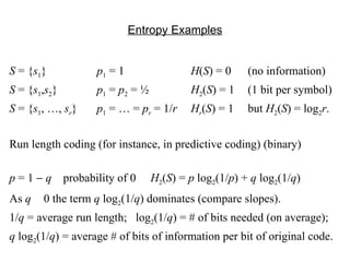
The document discusses entropy and Shannon's first theorem. It defines entropy as the average amount of information received per symbol from a source where symbols have different probabilities. Entropy measures the uncertainty in the probability distribution of the source. The entropy of a source is equal to the minimum expected code length needed to encode symbols from that source.

1. Chapter 6 Entropy and Shannon’s First Theorem

2. Information Axioms : I ( p ) = the amount of information in the occurrence of an event of probability p A. I ( p ) ≥ 0 for any event p B. I ( p 1 ∙ p 2 ) = I ( p 1 ) + I ( p 2 ) p 1 & p 2 are independent events C. I ( p ) is a continuous function of p Existence : I ( p ) = log_(1/ p ) units of information : in base 2 = a bit in base e = a nat in base 10 = a Hartley 6.2 A quantitative measure of the amount of information any probabilistic event represents. Cauchy functional equation source single symbol

3. Uniqueness : Suppose I ′( p ) satisfies the axioms. Since I ′( p ) ≥ 0, take any 0 < p 0 < 1, any base k = (1/ p 0 ) (1/ I′ ( p 0 )) . So k I′ ( p 0 ) = 1/ p 0 , and hence log k (1/ p 0 ) = I′ ( p 0 ). Now, any z  (0,1) can be written as p 0 r , r a real number  R + ( r = log p 0 z ). The Cauchy Functional Equation implies that I ′( p 0 n ) = n I ′( p 0 ) and m  Z + , I ′( p 0 1/ m ) = (1/ m ) I ′( p 0 ), which gives I ′( p 0 n / m ) = ( n / m ) I ′( p 0 ), and hence by continuity I ′( p 0 r ) = r I ′( p 0 ). Hence I ′( z ) = r ∙log k (1/ p 0 ) = log k (1/ p 0 r ) = log k (1/ z ).  Note : In this proof, we introduce an arbitrary p 0 , show how any z relates to it, and then eliminate the dependency on that particular p 0 . 6.2

4. Entropy The average amount of information received on a per symbol basis from a source S = { s 1 , …, s q } of symbols, s i has probability p i . It is measuring the rate . For radix r when all the probabilities are independent. Entropy is the amount of information in the probability distribution. Alternative approach: consider a long message of N symbols from S = { s 1 , …, s q } with probabilities p 1 , …, p q . You expect s i to appear Np i times, and the probability of this typical message is 6.3

5. Consider the function f ( p ) = p log (1/ p ). Use natural logarithms: f′ ( p ) = (- p log p ) ′ = - p (1/ p ) – log p = -1 + log (1/ p ) f ″ ( p ) = p (- p -2 ) = -1/ p < 0 for p  (0,1)  f is concave down f (1) = 0 1/ e f 0 1/ e 1 p 6.3 f ′(0) = ∞ f′ (1) = -1 f′ ( 1/ e ) = 0 f (1/ e ) = 1/ e

6. Gibbs Inequality Basic information about log function: Tangent line to y = ln x at x = 1 is ( y  ln 1) = (ln) ′ x =1 ( x  1)  y = x  1 (ln x )″ = (1/ x )′ = -(1/ x 2 ) < 0  x    ln x is concave down. Therefore, ln x  x  1 0 -1 1 ln x x y = x  1 6.4

7. Minimum Entropy occurs when one p i = 1 and all others are 0. Maximum Entropy occurs when? Consider Fundamental Gibbs inequality 6.4

8. Entropy Examples S = { s 1 } p 1 = 1 H ( S ) = 0 (no information) S = { s 1 , s 2 } p 1 = p 2 = ½ H 2 ( S ) = 1 (1 bit per symbol) S = { s 1 , …, s r } p 1 = … = p r = 1/ r H r ( S ) = 1 but H 2 ( S ) = log 2 r . Run length coding (for instance, in predictive coding) (binary) p = 1  q probability of 0 H 2 ( S ) = p log 2 (1/ p ) + q log 2 (1/ q ) As q  0 the term q log 2 (1/ q ) dominates (compare slopes). 1/ q = average run length; log 2 (1/ q ) = # of bits needed (on average); q log 2 (1/ q ) = average # of bits of information per bit of original code.

9. Entropy as a Lower Bound for Average Code Length Given an instantaneous code with length l i in radix r , let By the McMillan inequality, this hold for all uniquely decodable codes. Equality occurs when K = 1 (the decoding tree is complete) and 6.5

10. Shannon-Fano Coding The simplest variable length method. Less efficient than Huffman, but allows one to code symbol s i with length l i directly from p i . Given source symbols s 1 , …, s q with probabilities p 1 , …, p q pick l i =  log r (1/ p i )  . Hence, Summing this inequality over i : Kraft inequality is satisfied, therefore there is an instantaneous code with these lengths. 6.6

11. Example : p ’ s : ¼, ¼, ⅛, ⅛, ⅛, ⅛ l ’ s : 2, 2, 3, 3, 3, 3 K = 1 H 2 ( S ) = 2.5 L = 5/2 0 0 0 0 0 1 1 1 1 1 6.6

12. Recall: The n th extension of a source S = { s 1 , …, s q } with probabilities p 1 , …, p q is the set of symbols T = S n = { s i 1 ∙∙∙ s i n | s i j  S 1  j  n } where t i = s i 1 ∙∙∙ s i n has probability p i 1 ∙∙∙ p i n = Q i assuming independent probabilities. The entropy is: [Letting i = ( i 1 , …, i n ) q , an n -digit number base q ] The Entropy of Code Extensions concatenation multiplication 6.8

13. 6.8  H ( S n ) = n ∙ H ( S ) Hence the average S-F code length L n for T satisfies: H ( T )  L n < H ( T ) + 1  n ∙ H ( S )  L n < n ∙ H ( S ) + 1  H ( S )  ( L n / n ) < H ( S ) + 1/ n

14. Extension Example S = { s 1 , s 2 } p 1 = 2/3 p 2 = 1/3 H 2 ( S ) = (2/3)log 2 (3/2) + (1/3)log 2 (3/1) ~ 0.9182958 … Huffman coding: s 1 = 0 s 2 = 1 Avg. coded length = (2/3)∙1+(1/3)∙1 = 1 Shannon-Fano: l 1 = 1 l 2 = 2 Avg. coded length = (2/3)∙1+(1/3)∙2 = 4/3 2nd extention: p 11 = 4/9 p 12 = 2/9 = p 21 p 22 = 1/9 S-F : l 11 =  log 2 (9/4)  = 2 l 12 = l 21 =  log 2 (9/2)  = 3 l 22 =  log 2 (9/1)  = 4 L SF (2) = avg. coded length = (4/9)∙2+(2/9)∙3∙2+(1/9)∙4 = 24/9 = 2.666… S n = ( s 1 + s 2 ) n , whose probabilities are corresponding terms in ( p 1 + p 2 ) n 6.9

15. Extension cont. ( 2 + 1) n = 3 n 6.9 2 n 3 n -1 *

16. Markov Process Entropy 6.10

17. Example 6.11 0, 0 1, 0 0, 1 1, 1 .8 .8 .5 .5 .5 .5 .2 .2 equilibrium probabilities p (0,0) = 5/14 = p (1,1) p (0,1) = 2/14 = p (1,0) previous state next state S i 1 S i 2 S i p ( s i | s i 1 , s i 2 ) p ( s i 1 , s i 2 ) p ( s i 1 , s i 2 , s i ) 0 0 0 0.8 5/14 4/14 0 0 1 0.2 5/14 1/14 0 1 0 0.5 2/14 1/14 0 1 1 0.5 2/14 1/14 1 0 0 0.5 2/14 1/14 1 0 1 0.5 2/14 1/14 1 1 0 0.2 5/14 1/14 1 1 1 0.8 5/14 4/14

18. Base Fibonacci The golden ratio  = (1+√5)/2 is a solution to x 2 − x − 1 = 0 and is equal to the limit of the ratio of adjacent Fibonacci numbers. 0 … r − 1 H 2 = log 2 r 1/ r 0 1 1/  1/  2 1 0 1 st order Markov process: 0 10 1/  1/  2 1/  1/  2 1 0 1/  + 1/  2 = 1 Think of source as emitting variable length symbols: Entropy = (1/  )∙log  + ½ (1/  ² )∙log  ² = log  which is maximal take into account variable length symbols 1/  1/  2 0

19. The Adjoint System For simplicity, consider a first-order Markov system, S Goal: bound the entropy by a source with zero memory, yet whose probabilities are the equilibrium probabilities. Let p ( s i ) = equilibrium prob. of s i p ( s j ) = equilibrium prob. of s j p ( s j , s i ) = equilibrium probability of getting s j s i . with = only if p ( s j , s i ) = p ( s i ) · p ( s j ) Now, p ( s j , s i ) = p ( s i | s j ) · p ( s j ). = = = 6.12 (skip)