Download as PDF, PPTX
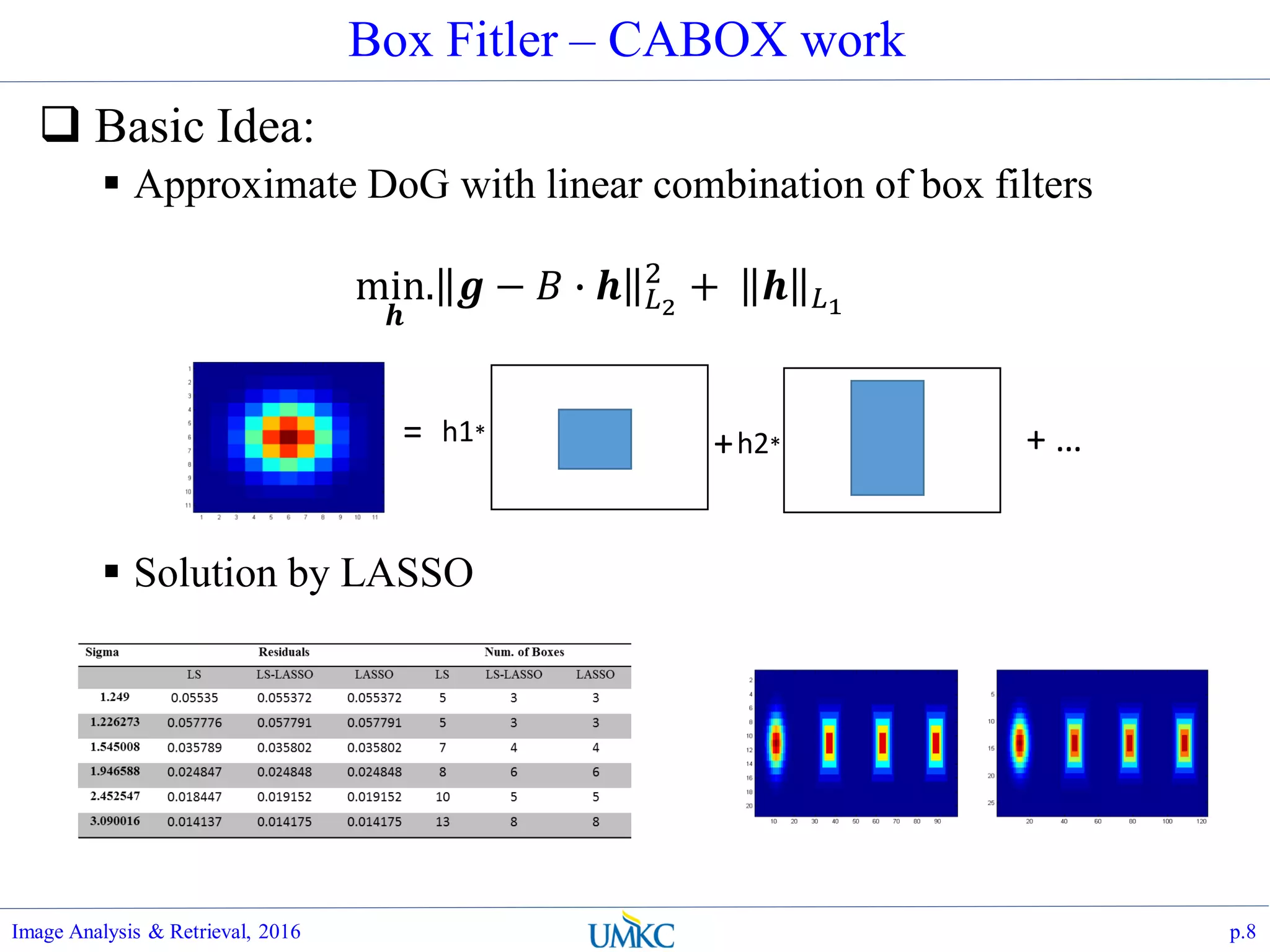
![Matlab Implementation
We will compute all image
pair distances D(j,k)
How do we compute the
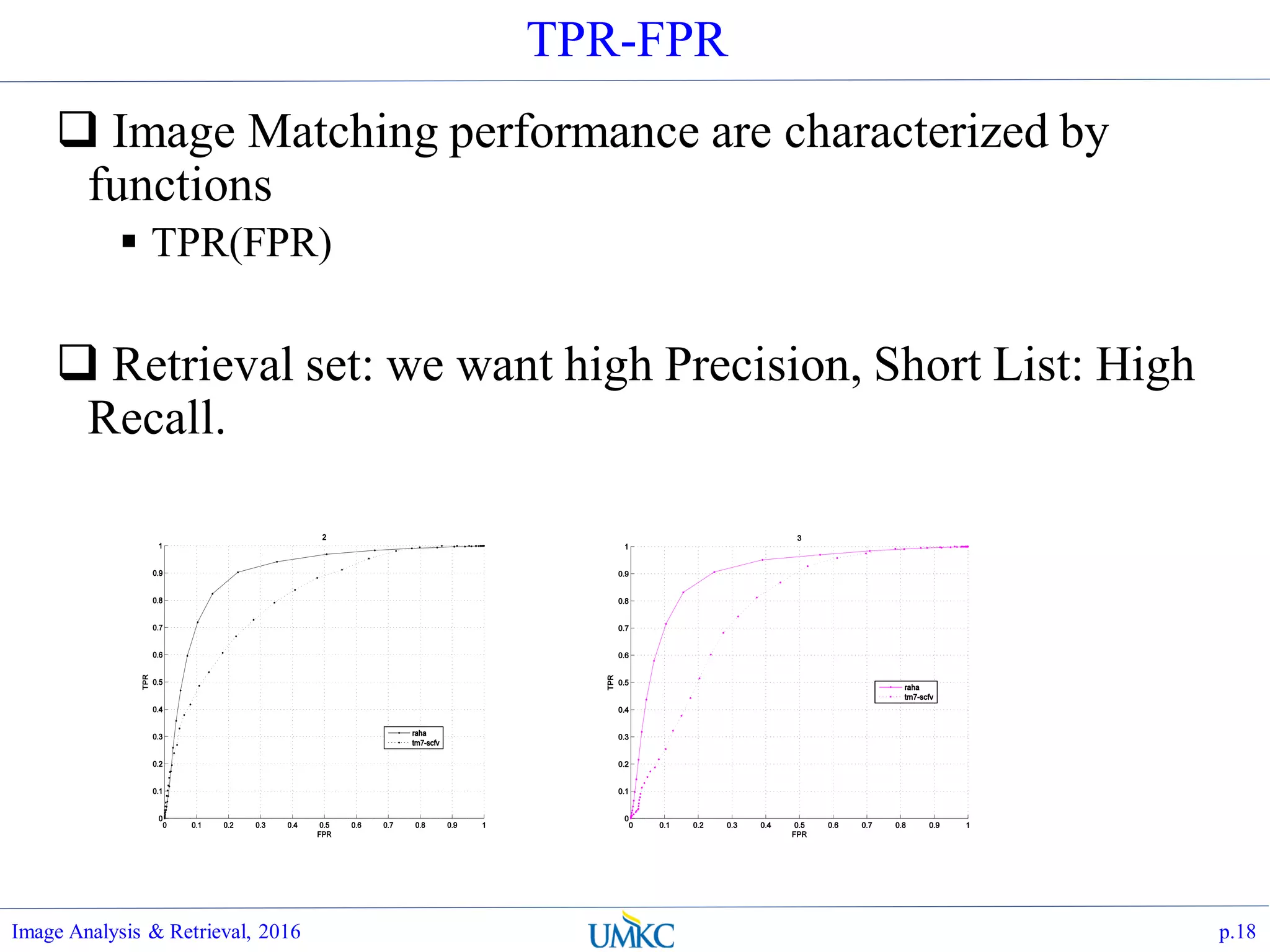
TPR-FPR plot ?
Understand that TPR and
FPR are actually function of
threshold t,
Just need to parameterize
TPR(t) and FPR(t), and
obtaining operating points of
meaningful thresholds, to
generate the plot.
Matlab Implementation:
[tp, fp, tn,
fn]=getPrecisionRecall()
Image Analysis & Retrieval, 2016 p.17
d_min = min(min(d0), min(d1));
d_max = max(max(d0), max(d1));
delta = (d_max - d_min) / npt;
for k=1:npt
thres = d_min + (k-1)*delta;
tp(k) = length(find(d0<=thres));
fp(k) = length(find(d1<=thres));
tn(k) = length(find(d1>thres));
fn(k) = length(find(d0>thres));
end
if dbg
figure(22); grid on; hold on;
plot(fp./(tn+fp), tp./(tp+fn), '.-r',
'DisplayName', 'tpr-fpr');legend();
end](https://image.slidesharecdn.com/lec07-aggregation-and-retrieval-system-161108175053/75/Lec07-aggregation-and-retrieval-system-17-2048.jpg)
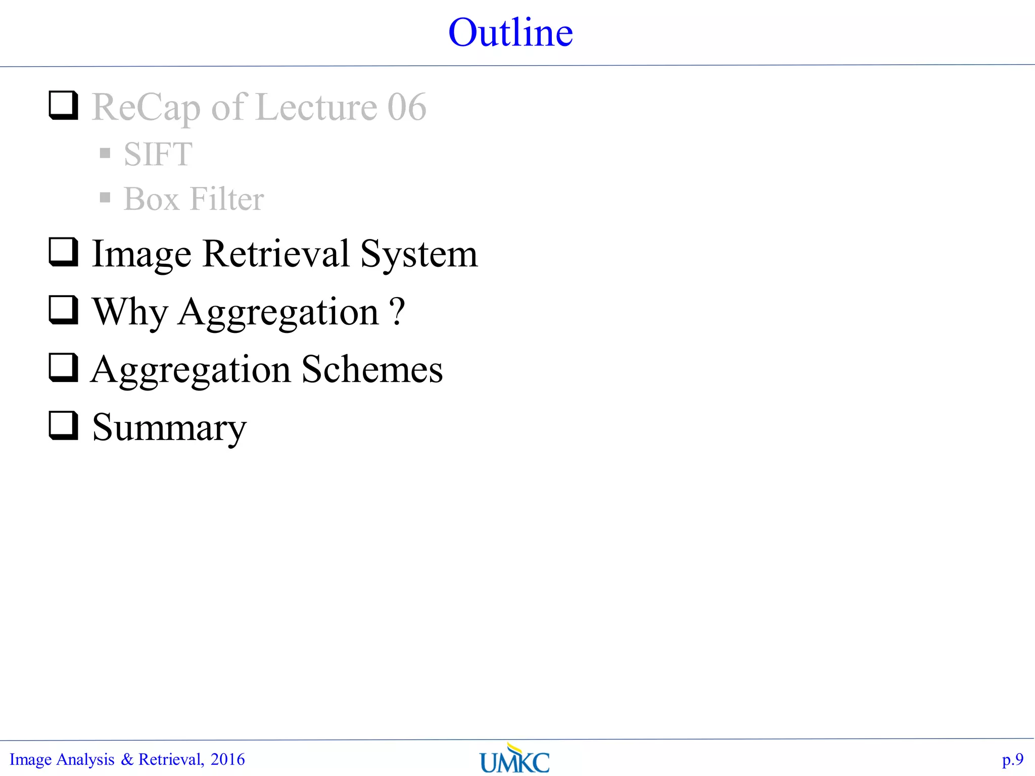
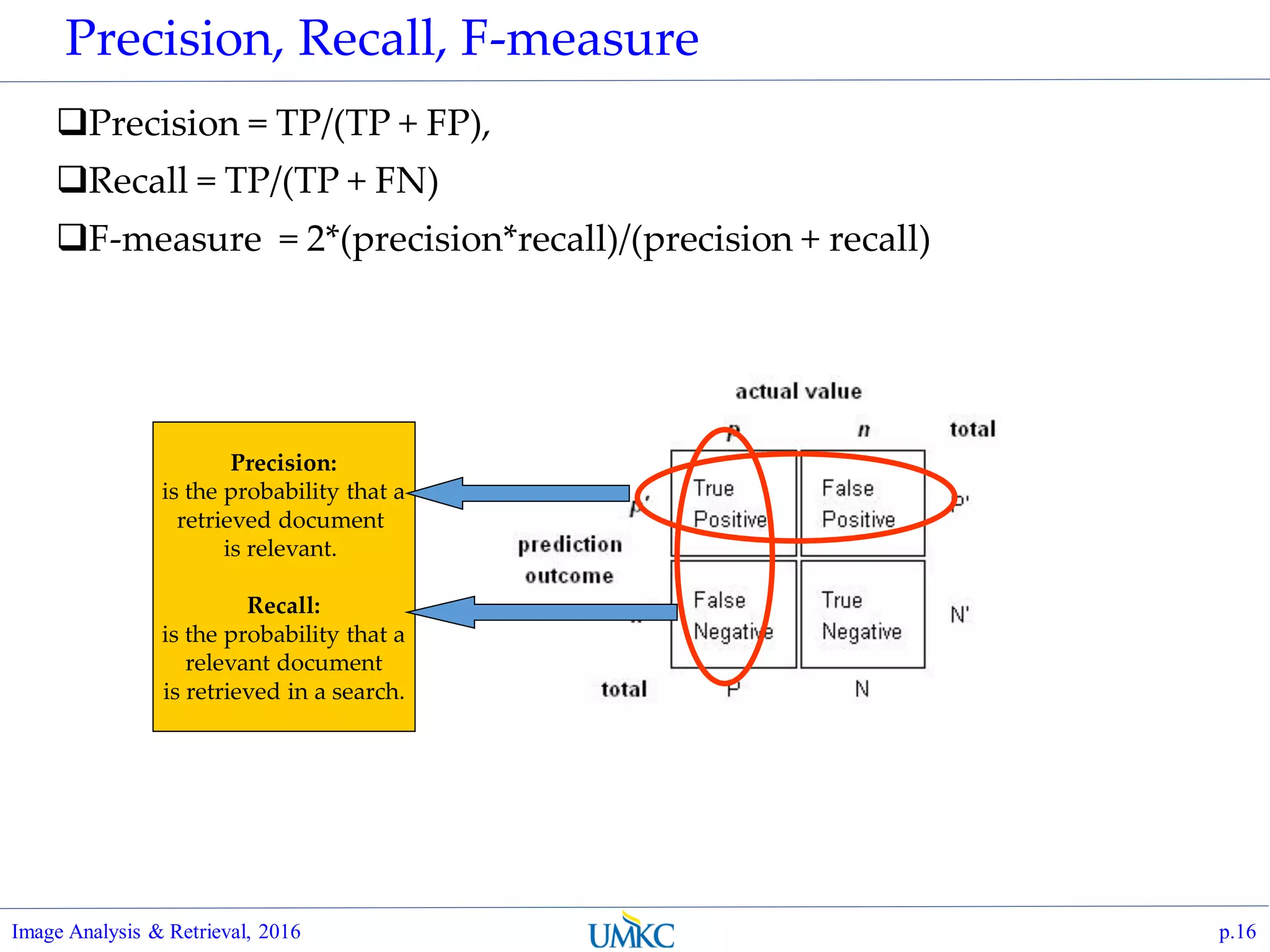
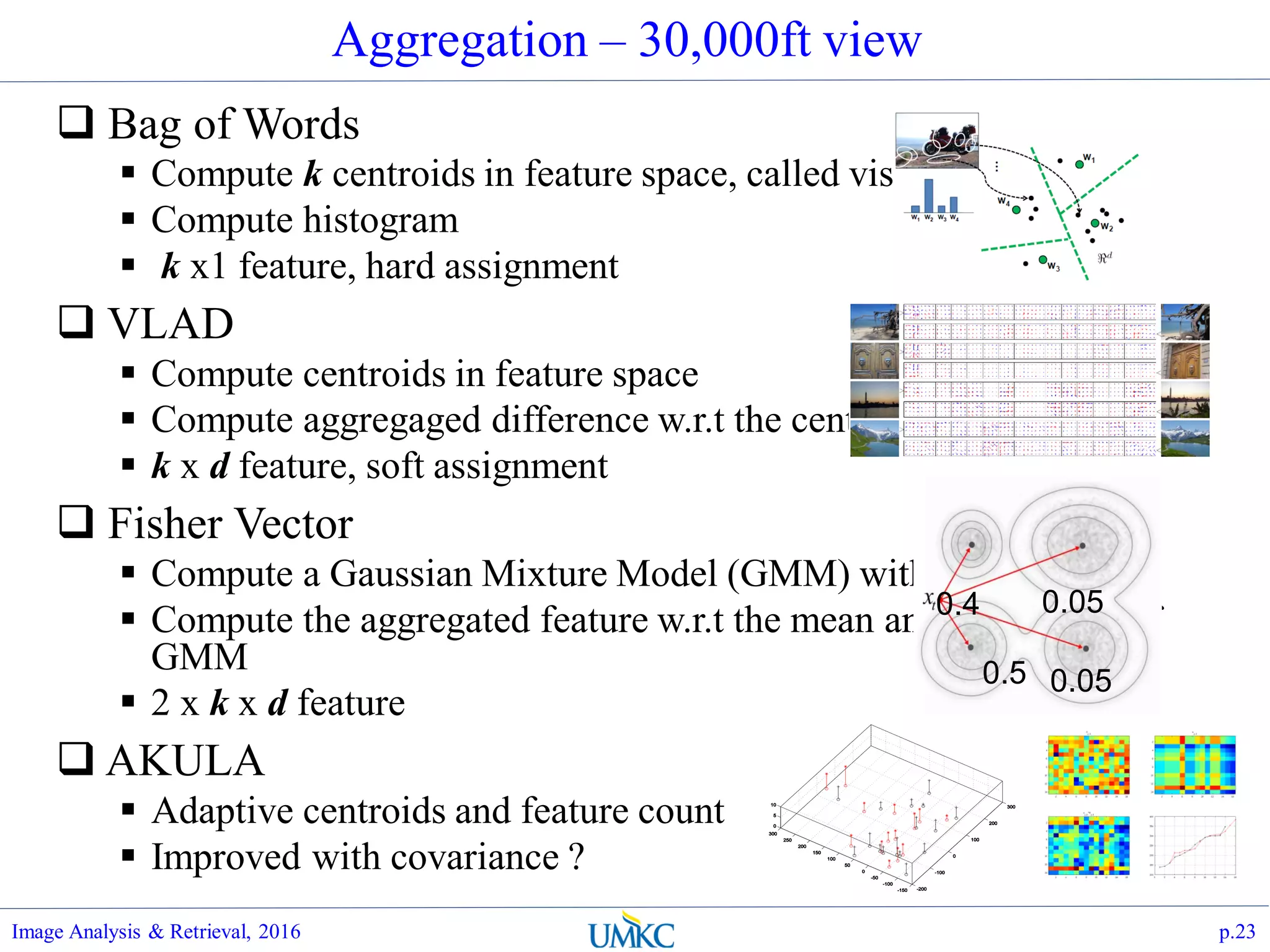
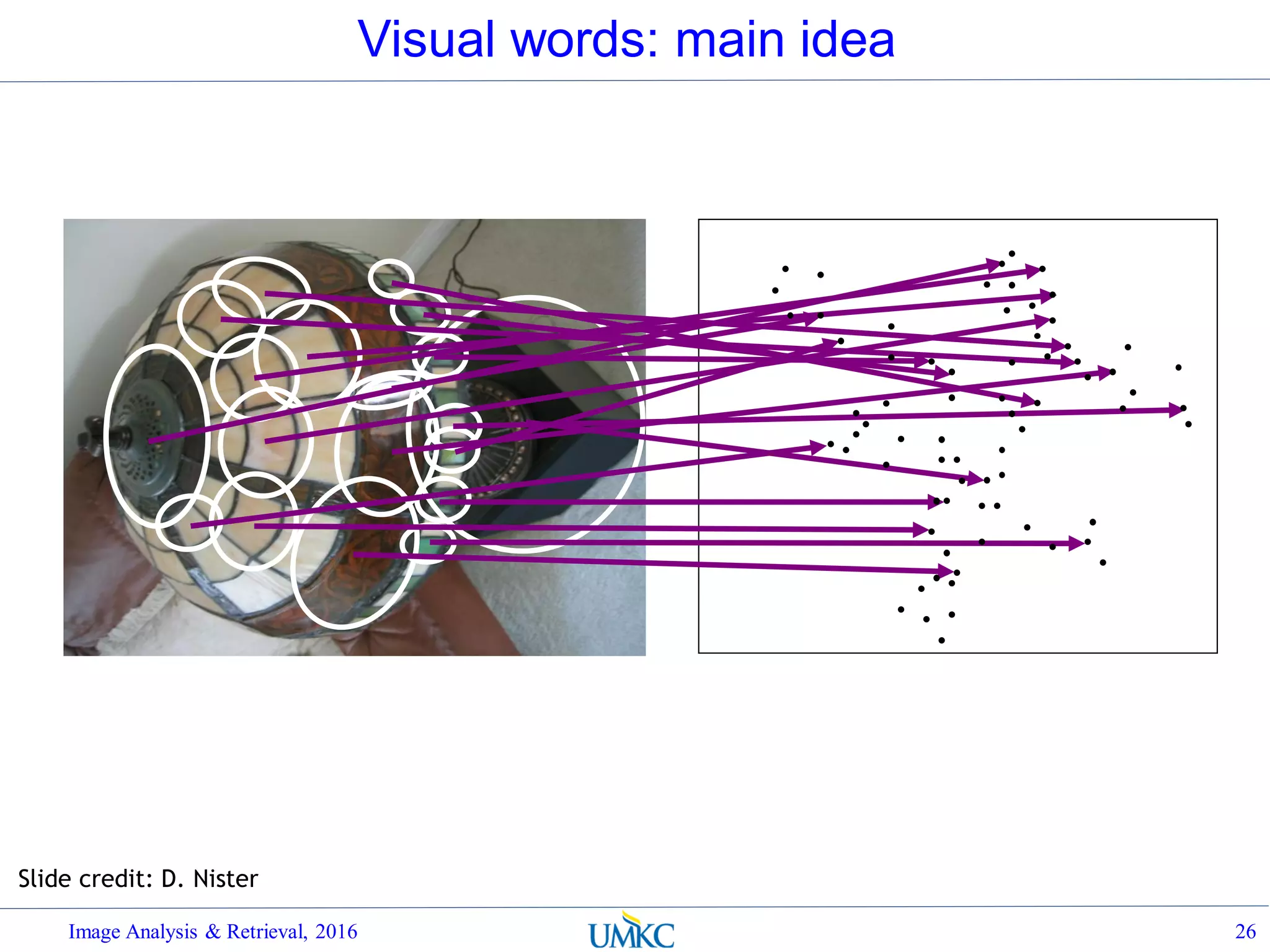
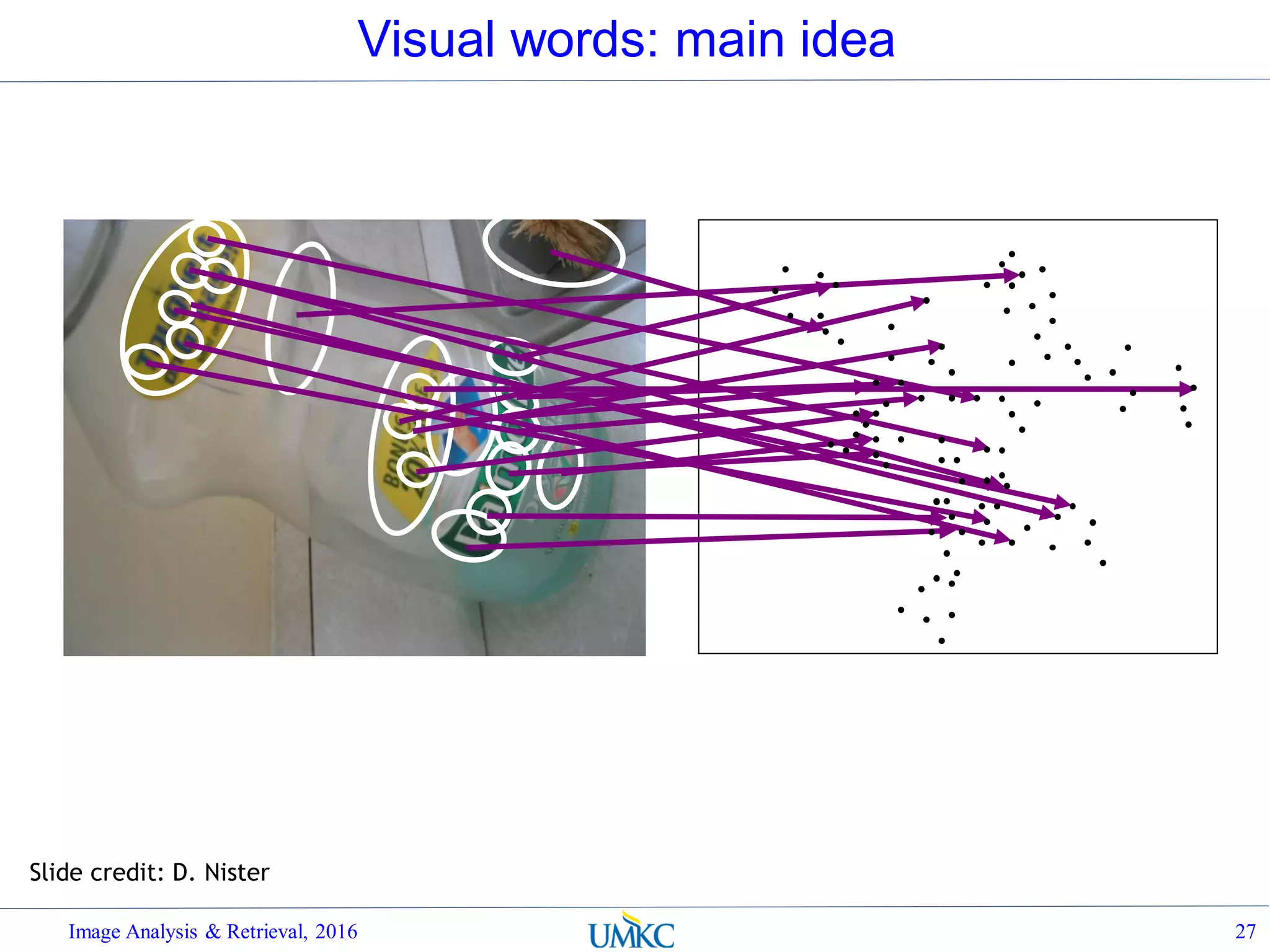
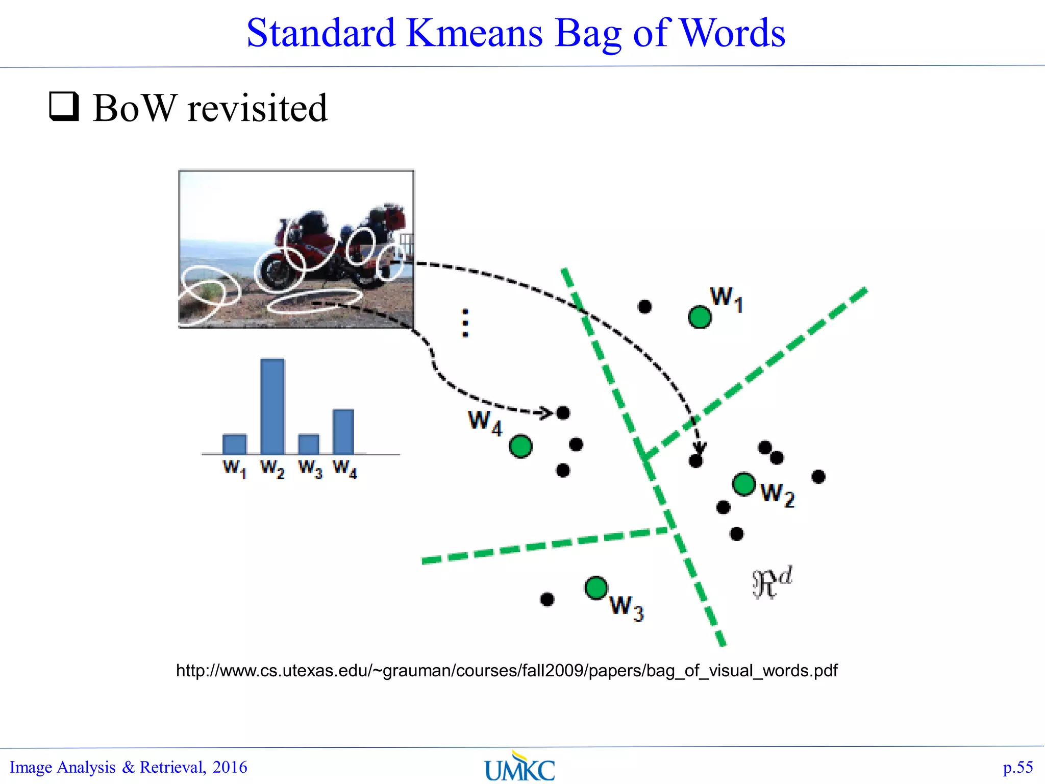
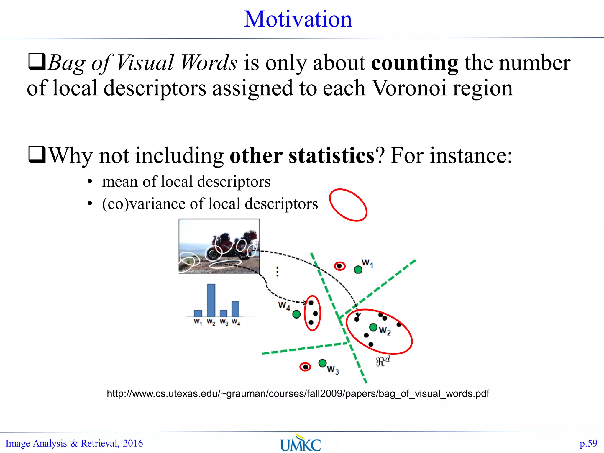
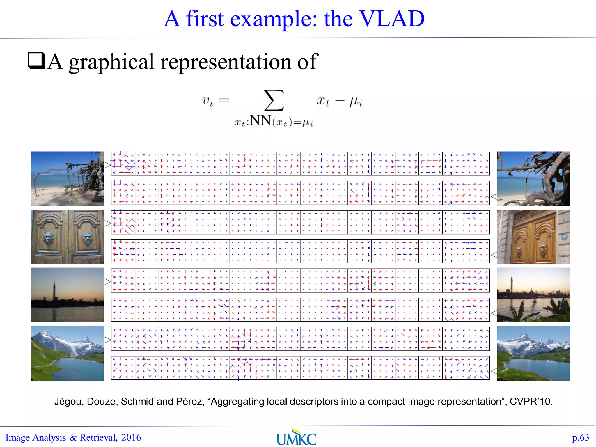
![Why Aggregation ?
What (Local) Interesting Points features bring us ?
Scale and rotation invariance in the form of nk x d:
Un-cerntainty of the number of detected features nk, at query
time
Permutation along rows of features are the same
representation.
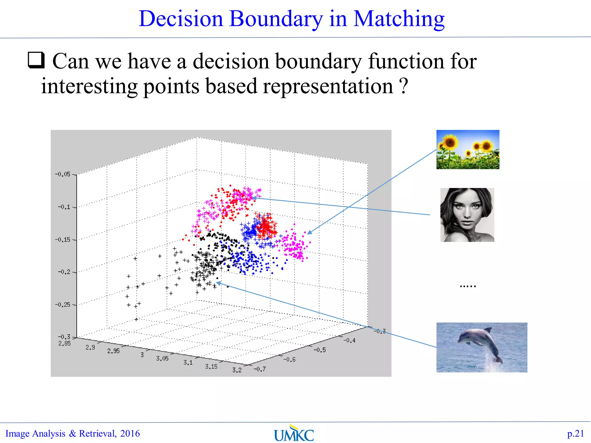
Problems:
The feature has state, not able to draw decision boundaries,
Not directly indexable/hashable
Typically very high dimensionality
Image Analysis & Retrieval, 2016 p.20
𝑆 𝑘| [𝑥 𝑘, 𝑦 𝑘, 𝜃 𝑘, 𝜎 𝑘, ℎ1, ℎ2, … , ℎ128] , 𝑘 = 1. . 𝑛](https://image.slidesharecdn.com/lec07-aggregation-and-retrieval-system-161108175053/75/Lec07-aggregation-and-retrieval-system-20-2048.jpg)
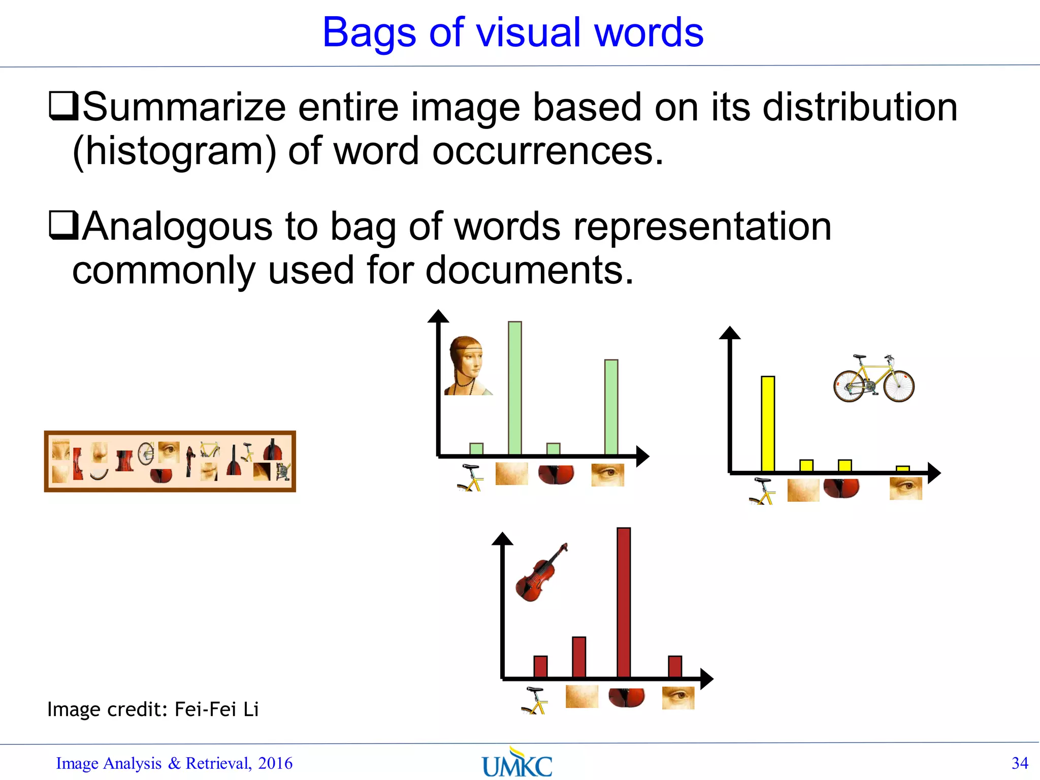
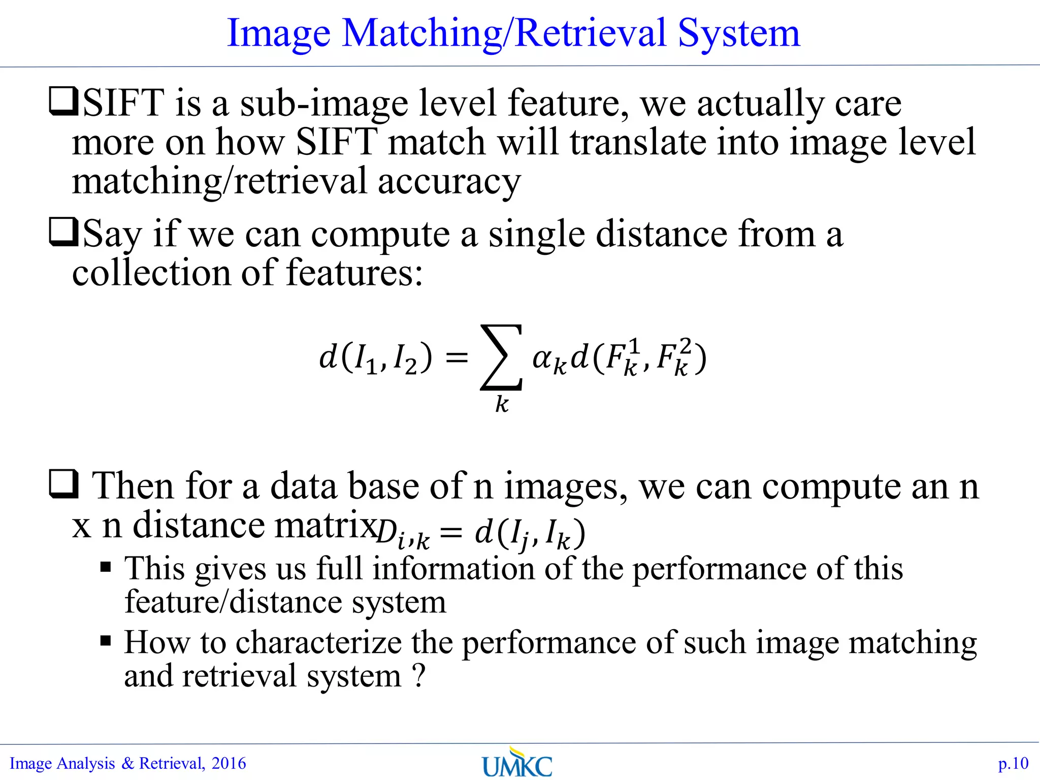
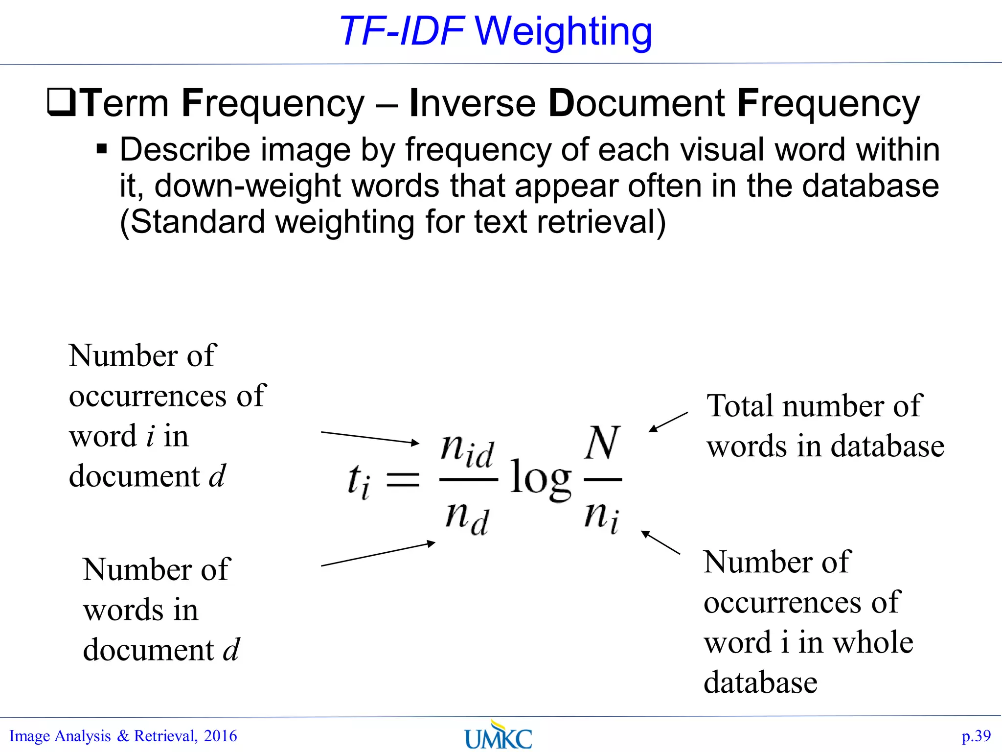
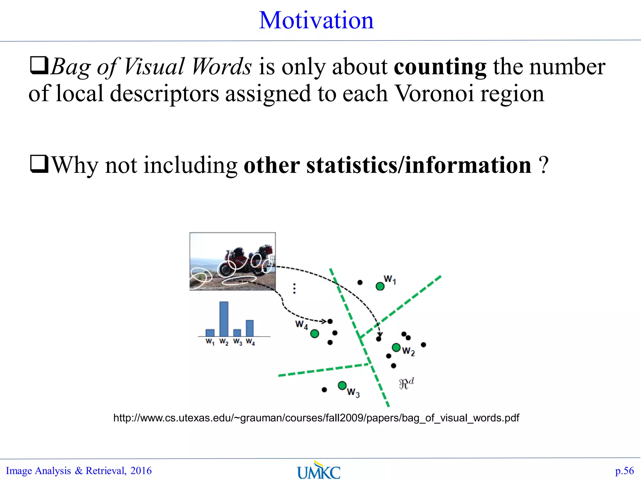
![BoW Distance Metrics
Rank images by normalized scalar product
between their (possibly weighted) occurrence
counts---nearest neighbor search for similar
images.
Image Analysis & Retrieval, 2016 p.36
[5 1 1 0][1 8 1 4]
dj
q](https://image.slidesharecdn.com/lec07-aggregation-and-retrieval-system-161108175053/75/Lec07-aggregation-and-retrieval-system-36-2048.jpg)
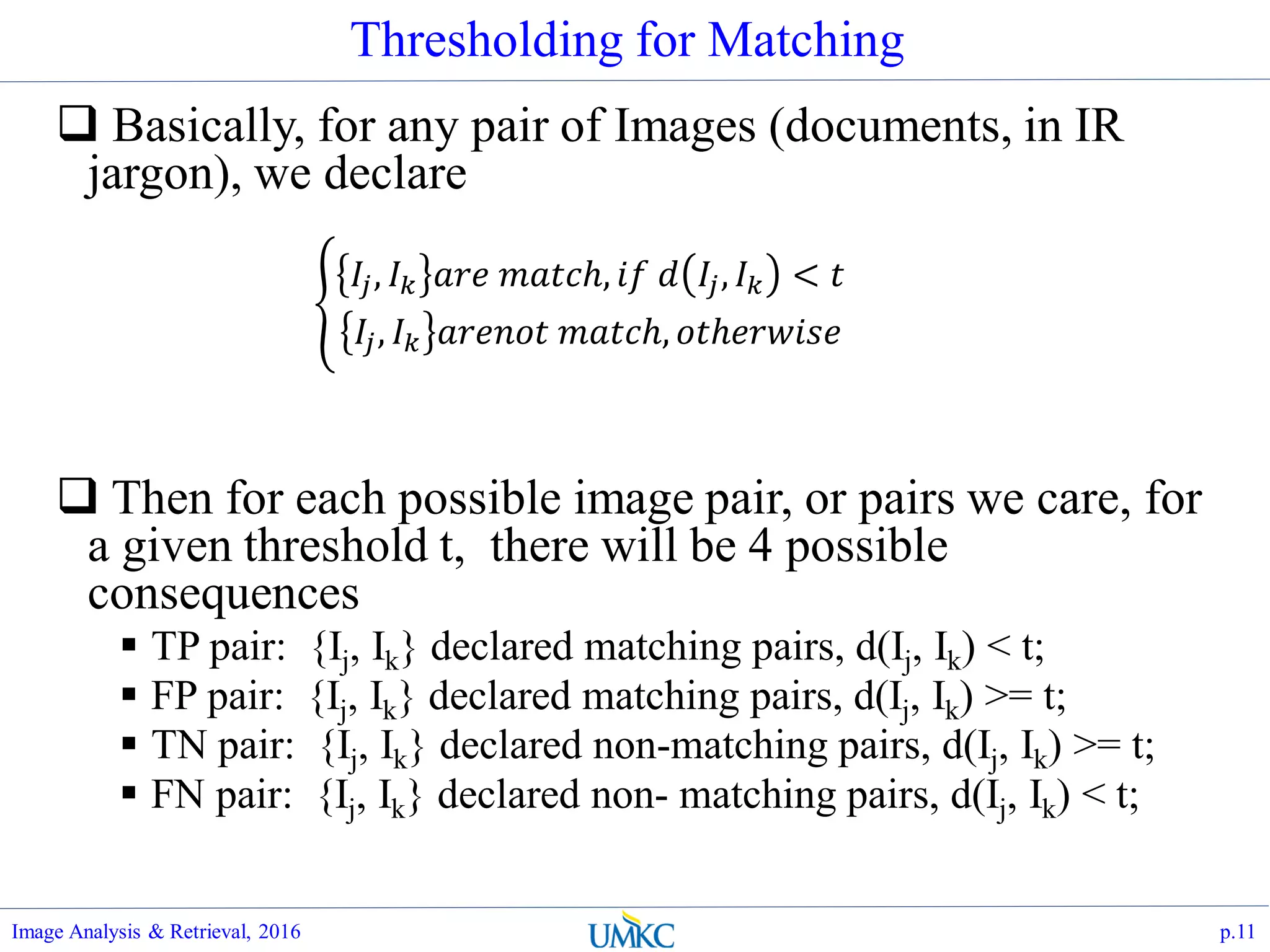
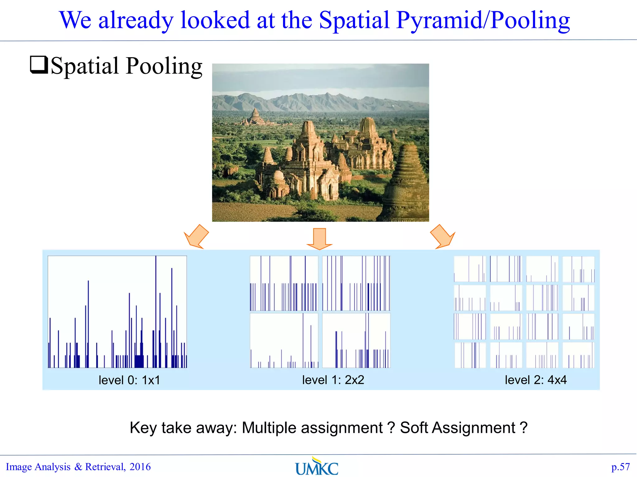
![Hiearchical Assignment of Histogram
Tree construction:
Image Analysis & Retrieval, 2016 44
[Nister & Stewenius, CVPR’06]](https://image.slidesharecdn.com/lec07-aggregation-and-retrieval-system-161108175053/75/Lec07-aggregation-and-retrieval-system-44-2048.jpg)
![Vocabulary Tree
Training: Filling the tree
Image Analysis & Retrieval, 2016 45
[Nister & Stewenius, CVPR’06]](https://image.slidesharecdn.com/lec07-aggregation-and-retrieval-system-161108175053/75/Lec07-aggregation-and-retrieval-system-45-2048.jpg)
![46
Vocabulary Tree
Training: Filling the tree
Image Analysis & Retrieval, 2016 46Slide credit: David Nister
[Nister & Stewenius, CVPR’06]](https://image.slidesharecdn.com/lec07-aggregation-and-retrieval-system-161108175053/75/Lec07-aggregation-and-retrieval-system-46-2048.jpg)
![47
Vocabulary Tree
Training: Filling the tree
Image Analysis & Retrieval, 2016 47Slide credit: David Nister
[Nister & Stewenius, CVPR’06]](https://image.slidesharecdn.com/lec07-aggregation-and-retrieval-system-161108175053/75/Lec07-aggregation-and-retrieval-system-47-2048.jpg)
![Vocabulary Tree
Training: Filling the tree
Image Analysis & Retrieval, 2016 48
[Nister & Stewenius, CVPR’06]](https://image.slidesharecdn.com/lec07-aggregation-and-retrieval-system-161108175053/75/Lec07-aggregation-and-retrieval-system-48-2048.jpg)
![Vocabulary Tree
Training: Filling the tree
Image Analysis & Retrieval, 2016 49
[Nister & Stewenius, CVPR’06]](https://image.slidesharecdn.com/lec07-aggregation-and-retrieval-system-161108175053/75/Lec07-aggregation-and-retrieval-system-49-2048.jpg)
![50
Vocabulary Tree
Recognition
Image Analysis & Retrieval, 2016 50Slide credit: David Nister
[Nister & Stewenius, CVPR’06]
RANSAC
verification](https://image.slidesharecdn.com/lec07-aggregation-and-retrieval-system-161108175053/75/Lec07-aggregation-and-retrieval-system-50-2048.jpg)
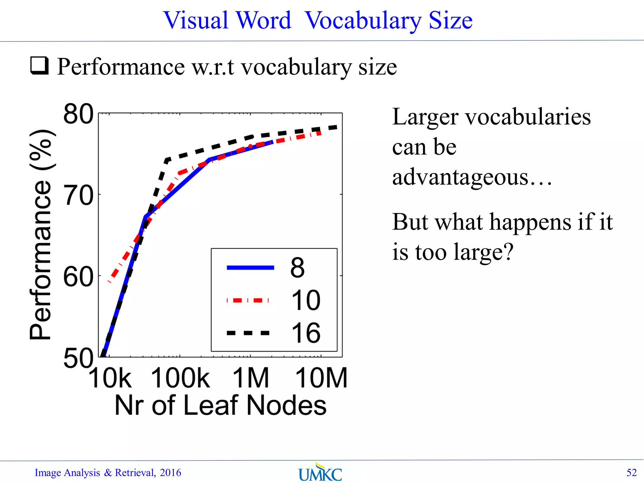
![Vocabulary Tree: Performance
Evaluated on large databases
Indexing with up to 1M images
Online recognition for database
of 50,000 CD covers
Retrieval in ~1s
Find experimentally that large vocabularies can be
beneficial for recognition
Image Analysis & Retrieval, 2016 51
[Nister & Stewenius, CVPR’06]](https://image.slidesharecdn.com/lec07-aggregation-and-retrieval-system-161108175053/75/Lec07-aggregation-and-retrieval-system-51-2048.jpg)
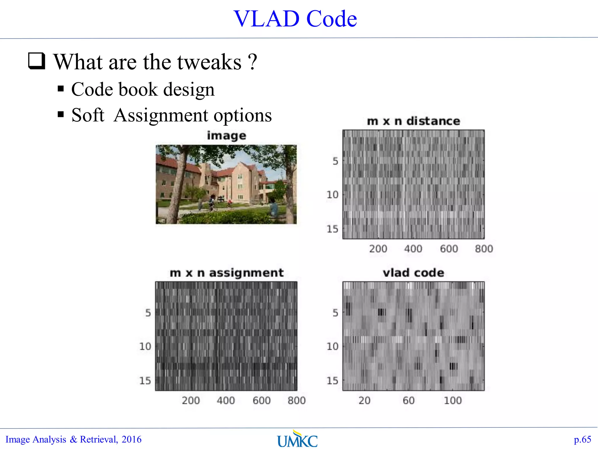
![VL_FEAT Implementation
Matlab:
Image Analysis & Retrieval, 2016 p.64
function [vc]=vladSiftEncoding(sift,
codebook)
dbg=1;
if dbg
if (0) % init VL_FEAT, only need
to do once
run('../../tools/vlfeat-
0.9.20/toolbox/vl_setup.m');
end
im = imread('../pics/flarsheim-
2.jpg');
[f, sift] =
vl_sift(single(rgb2gray(im))); sift =
single(sift');
[indx, codebook] = kmeans(sift,
16);
% make sift # smaller
sift = sift(1:800,:);
end
[n, kd]=size(sift);
[m, kd]=size(codebook);
% compute assignment
dist = pdist2(codebook, sift);
mdist = mean(mean(dist));
% normalize the heat kernel s.t. mean
dist is mapped to 0.5
a = -log(0.5)/mdist;
indx = exp(-a*dist);
vc=vl_vlad(sift', codebook', indx);
if dbg
figure(41); colormap(gray);
subplot(2,2,1); imshow(im);
title('image');
subplot(2,2,2); imagesc(dist);
title('m x n distance');
subplot(2,2,3); imagesc(indx);
title('m x n assignment');
subplot(2,2,4); imagesc(reshape(vc,
[m, kd]));title('vlad code');
end](https://image.slidesharecdn.com/lec07-aggregation-and-retrieval-system-161108175053/75/Lec07-aggregation-and-retrieval-system-64-2048.jpg)

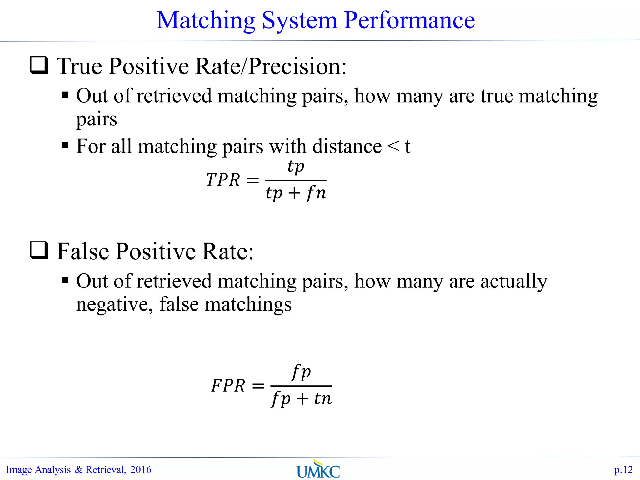
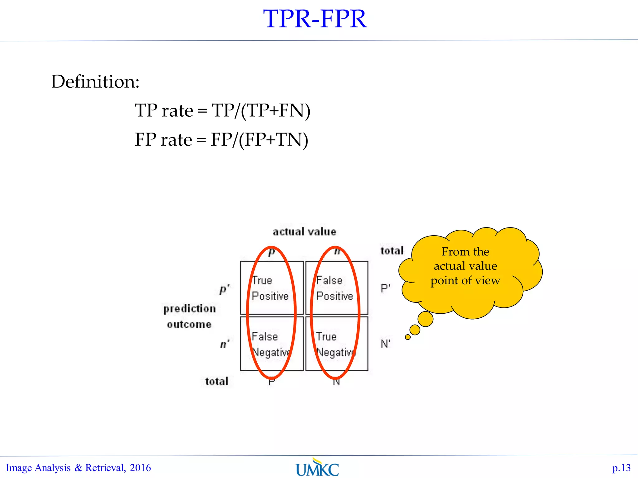
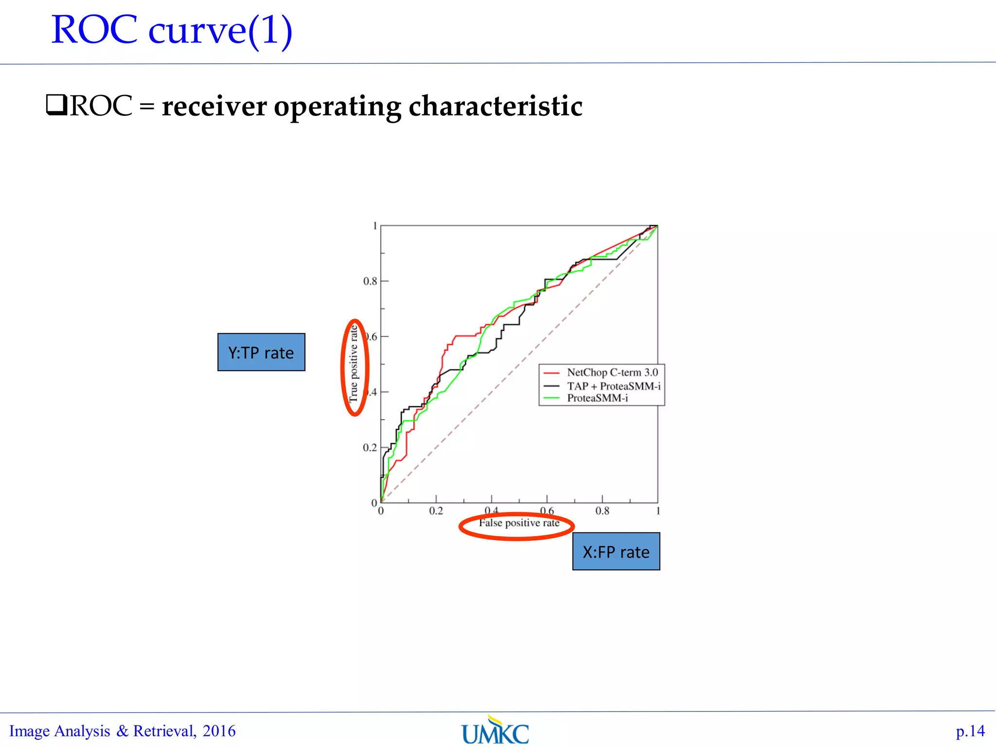
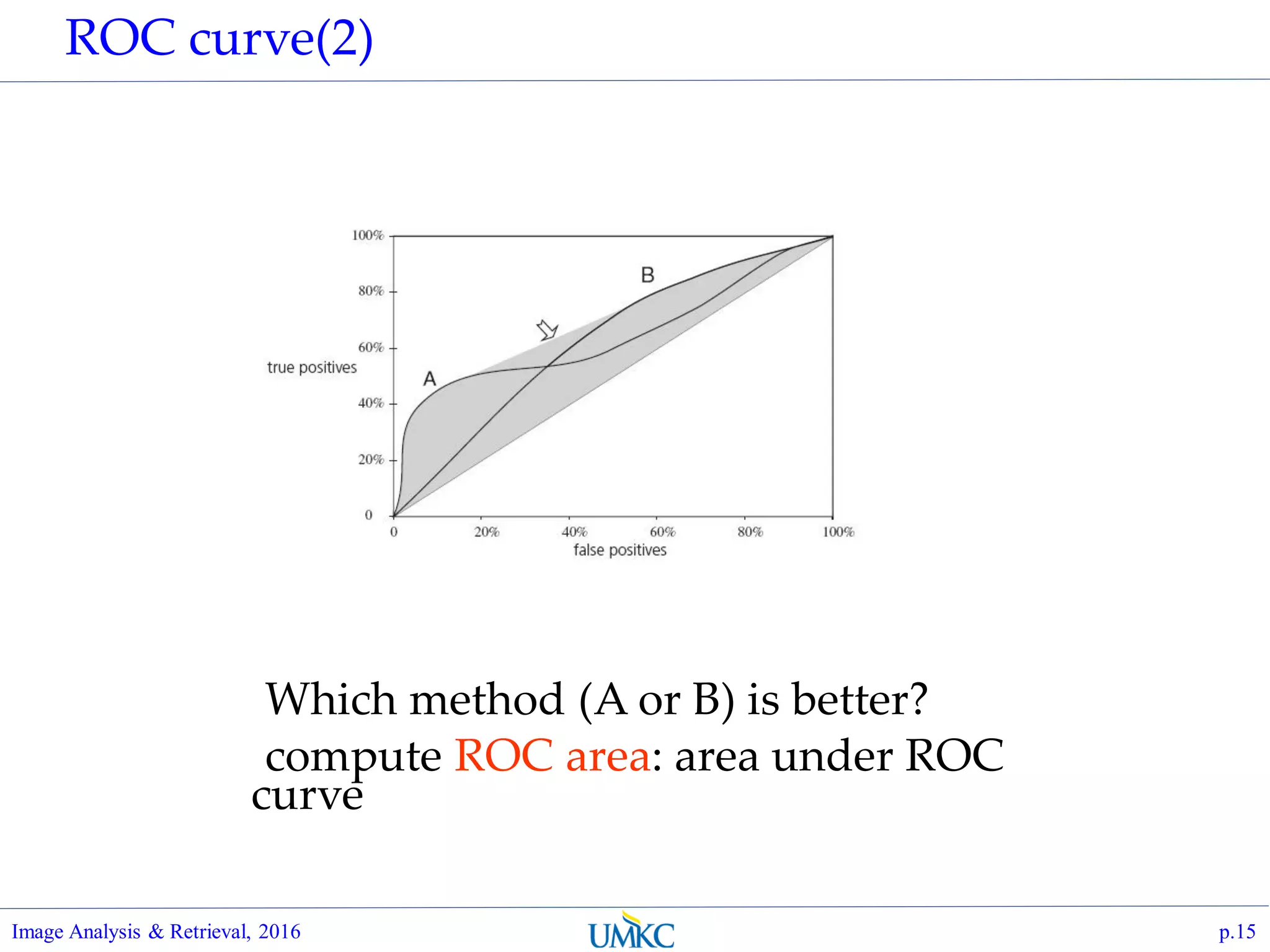
The document outlines a lecture on image analysis and retrieval, focusing on SIFT (Scale-Invariant Feature Transform) and box filtering techniques for image feature extraction and matching. It discusses the importance of feature aggregation for improved retrieval accuracy, introduces various aggregation methods, and examines performance metrics such as precision, recall, and ROC curves. Additionally, it covers practical implementations and challenges in high-dimensional feature spaces and the bag-of-words model for image classification.