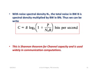
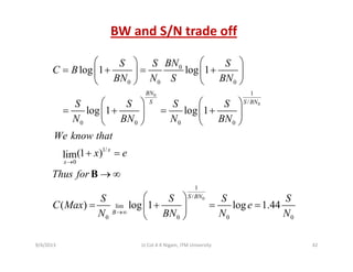
Download as PDF, PPTX
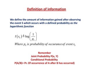

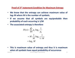
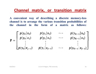
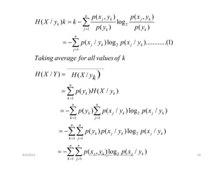
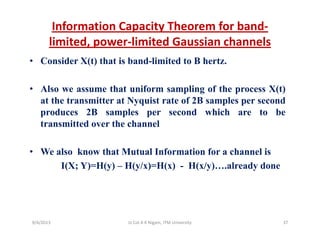
![• We know that I(x, y)=H(y)‐H(y/x)……..1
Solution
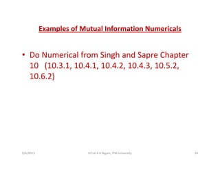
We know that I(x, y) H(y) H(y/x)……..1
• Finding H(y)
• P(y1)=0.6×0.8+.4×0.3=.6
• P(y2)=0.6×0.2+0.4×0.7=.4
• H(y)=‐3.322× [0.6log0.6+0.4log0.4]=0.971 bits/message
• Finding H(y/x)= ‐
• Finding P(x, y)
( , )log ( / )p x y p y x∑∑
48 12⎡ ⎤
• H(y/x)= ‐3 322[0 48×log0 8+0 12×log0 2+ 0 12×logo 3+0 28×log0 7]
.48 .12
( , )
.12 .28
P x y
⎡ ⎤
= ⎢ ⎥
⎣ ⎦
• H(y/x)= ‐3.322[0.48×log0.8+0.12×log0.2+ 0.12×logo.3+0.28×log0.7]
= 0.7852
• Putting values in 1 we get I(x, y)=0.971‐0.7852=0.1858 bitsg g ( , y)
9/4/2013 26Lt Col A K Nigam, ITM University](https://image.slidesharecdn.com/dcsunit2-140609034947-phpapp02/85/Dcs-unit-2-26-320.jpg)
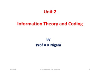
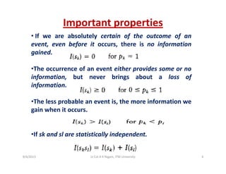
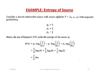
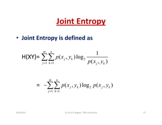
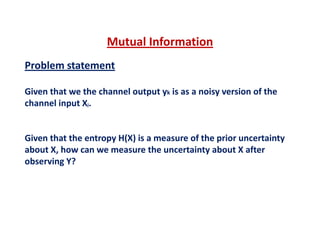
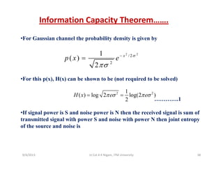
![Lossless channel
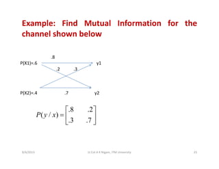
• For a lossless channel no source information is lost in
transmission. It has only one non zero element in each
column For examplecolumn. For example
[ ]
3/ 4 1/ 4 0 0 0
( / ) 0 0 1/ 3 2 / 3 0P Y X
⎡ ⎤
⎢ ⎥
⎢ ⎥
• In case of lossless channel p(x/y)=0/1 as the probability of x
[ ]( / ) 0 0 1/ 3 2 / 3 0
0 0 0 0 1
P Y X = ⎢ ⎥
⎢ ⎥⎣ ⎦
• In case of lossless channel p(x/y)=0/1 as the probability of x
given that y has occurred is 0/1
• Putting this in eq 3 we get H(x/y)=0
• Thus from eq. 1 we get
I(x, y)=H(x)
Also C=max H(x)Also C=max H(x)
9/4/2013 29Lt Col A K Nigam, ITM University](https://image.slidesharecdn.com/dcsunit2-140609034947-phpapp02/85/Dcs-unit-2-29-320.jpg)
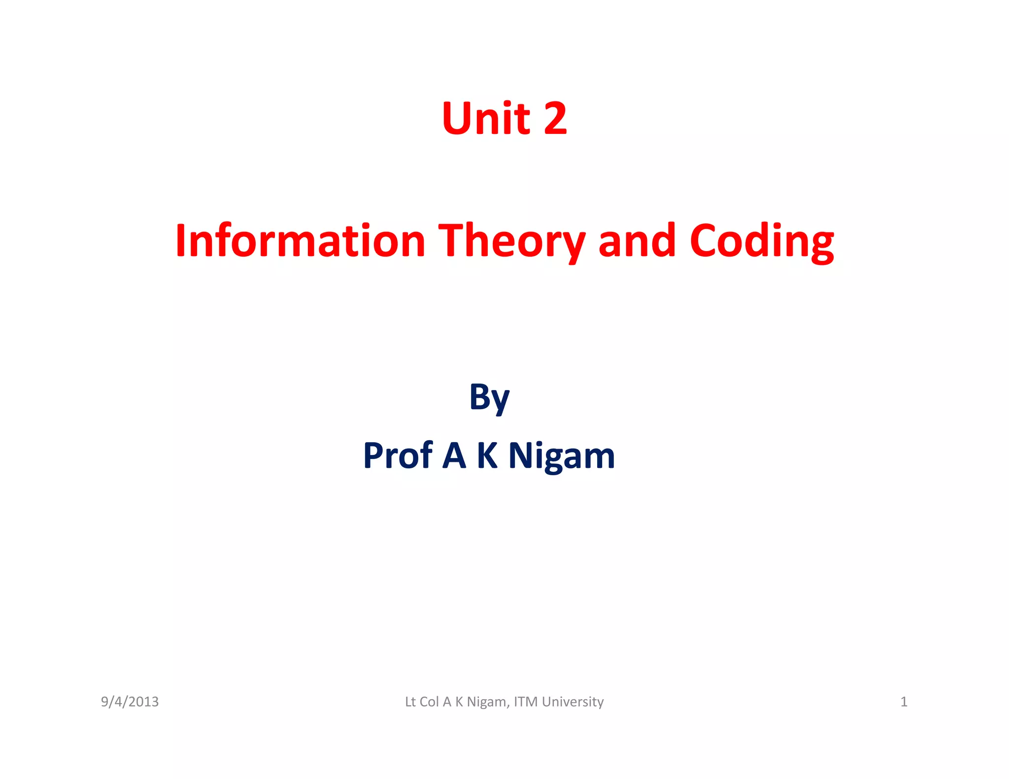
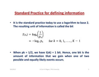
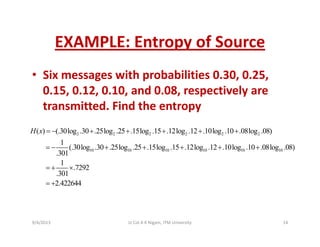
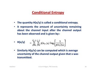
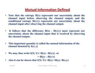
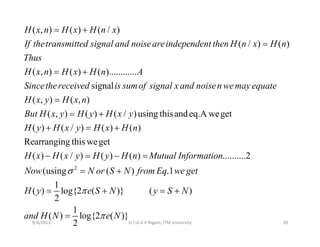
![Deterministic channel
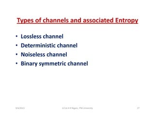
• Channel matrix has only one non zero element in each row, for
example
1 0 0
1 0 0
⎡ ⎤
⎢ ⎥
⎢ ⎥
[ ]
1 0 0
( / ) 0 1 0
0 1 0
0 0 1
P Y X
⎢ ⎥
⎢ ⎥=
⎢ ⎥
⎢ ⎥
⎢ ⎥⎣ ⎦
• In case of Deterministic channel p(y/x)=0/1 as the probability of y
given that x has occurred is 0/1
0 0 1⎢ ⎥⎣ ⎦
• Putting this in eq 3 we get H(y/x)=0
• Thus from eq. 1 we get
I(x, y)=H(y)
Also C=max H(y)
9/4/2013 30Lt Col A K Nigam, ITM University](https://image.slidesharecdn.com/dcsunit2-140609034947-phpapp02/85/Dcs-unit-2-30-320.jpg)
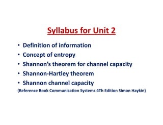
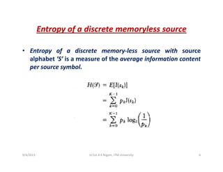
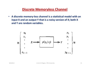
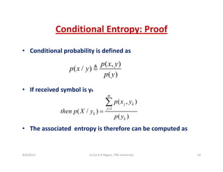
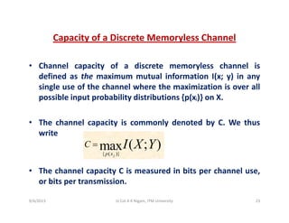
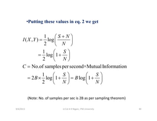
![Noiseless channel
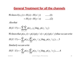
• A channel which is both lossless and deterministic, has only one
element in each row and column. For example
1 0 0 0⎡ ⎤
[ ]
1 0 0 0
0 1 0 0
( / )
0 0 1 0
P y x
⎡ ⎤
⎢ ⎥
⎢ ⎥=
⎢ ⎥
• Noiseless channel is both lossless and deterministic thus
H( / ) H( / ) 0
0 0 1 0
0 0 0 1
⎢ ⎥
⎢ ⎥
⎣ ⎦
H(x/y)=H(y/x)=0
• Thus from eq. 1 we get
I(x, y)=H(y)=H(x)
Also C=max H(y)=max H(x)=log2m=log2n where m and n areAlso C=max H(y)=max H(x)=log2m=log2n where m and n are
number of symbols
9/4/2013 31Lt Col A K Nigam, ITM University](https://image.slidesharecdn.com/dcsunit2-140609034947-phpapp02/85/Dcs-unit-2-31-320.jpg)
![2
1 1
( / ) ( , )log ( / )
n n
j k k j
k j
H Y Y p x y p y x
= =
= −∑∑
( / ) [ (1 )log(1 ) log (1 ) log
putting values frommatrix we get
H Y Y p p p p p pα α α= − − − + + −
(1 )(1 )log(1 )]
[ log (1 )log(1 )]
p p
p p p p
α− − −
= − + − −
.1
( , ) ( ) log (1 )log(1
Putting thisineq we get
I X Y H y p p p= + + − − )p
9/4/2013 33Lt Col A K Nigam, ITM University](https://image.slidesharecdn.com/dcsunit2-140609034947-phpapp02/85/Dcs-unit-2-33-320.jpg)

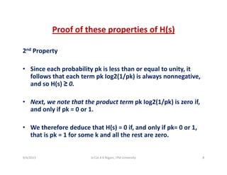
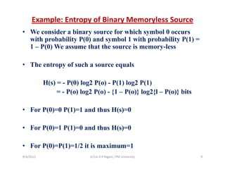
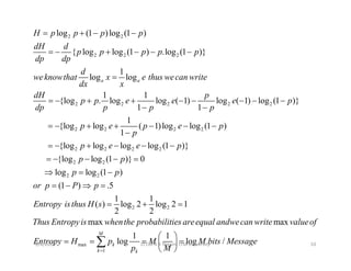
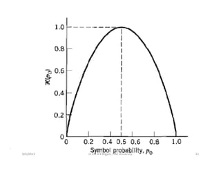
This document provides an overview of information theory and coding concepts including: 1) Definitions of information, entropy, joint entropy, conditional entropy, and mutual information are introduced along with examples of calculating these quantities for discrete memoryless sources and channels. 2) Shannon's theorem for channel capacity is discussed and the channel capacity of a discrete memoryless channel is defined as the maximum mutual information over all possible input distributions. 3) Properties of entropy such as it being a measure of uncertainty, having a minimum of 0 and maximum of log2K, and being maximized when probabilities are equal are proven.