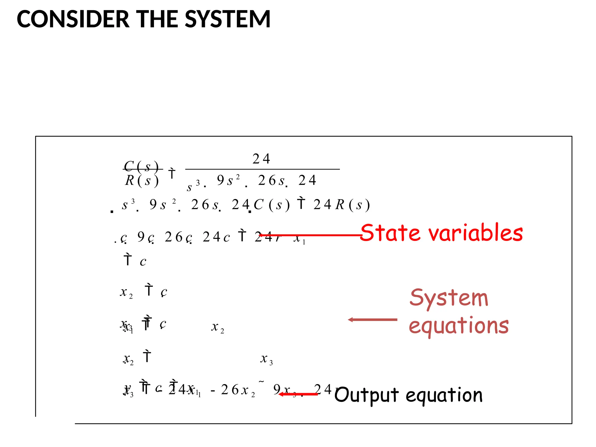
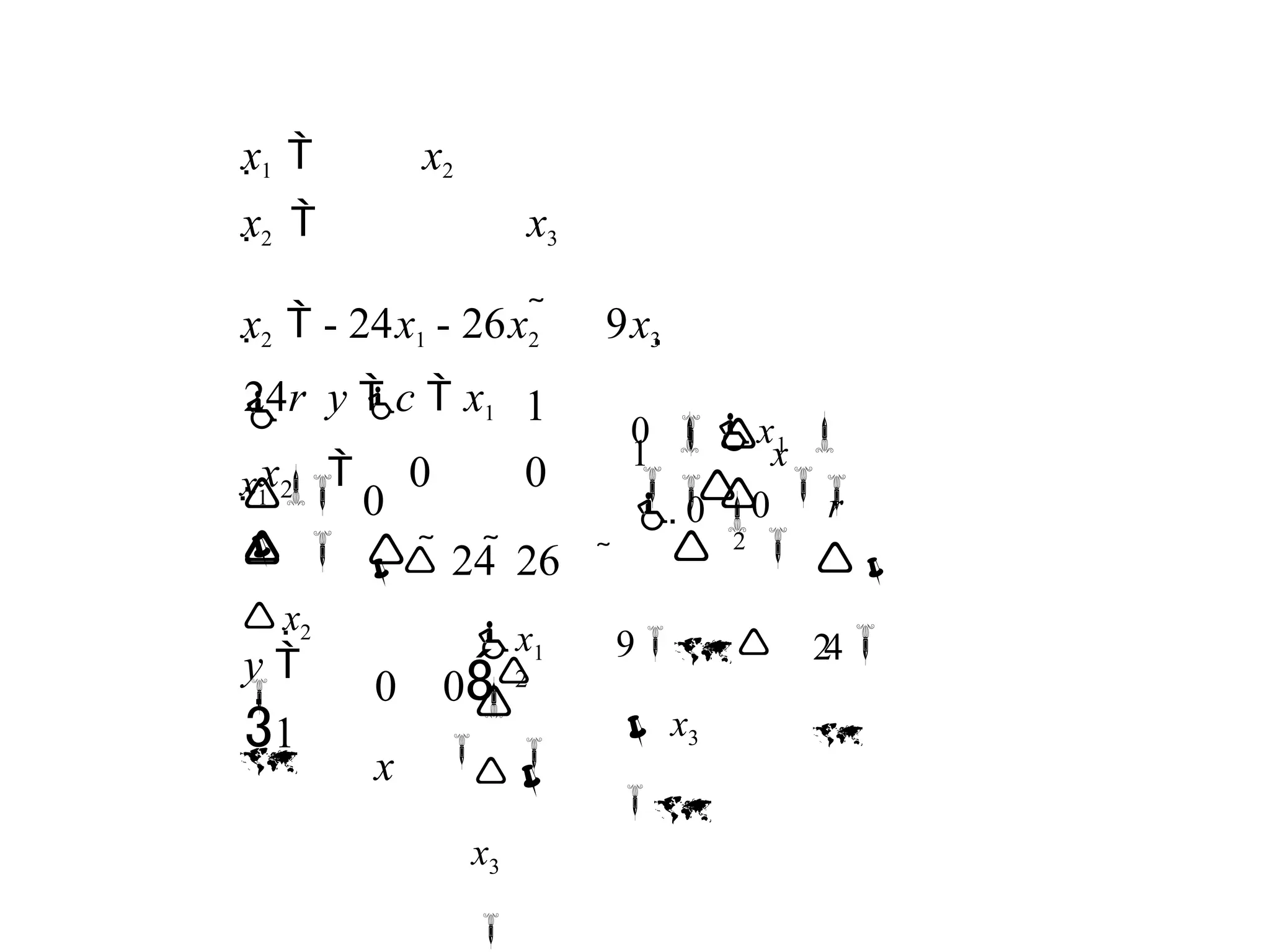
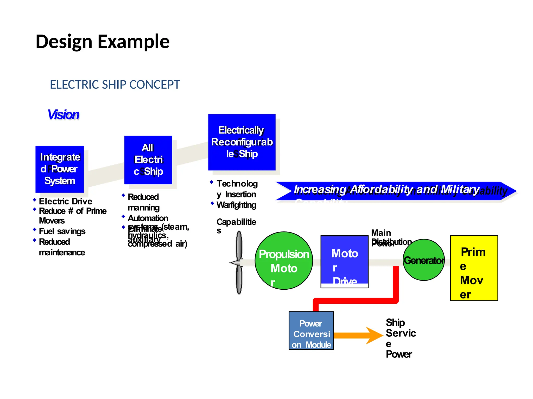
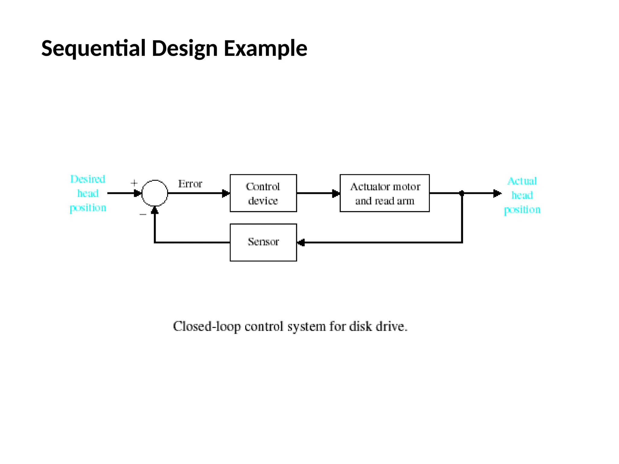
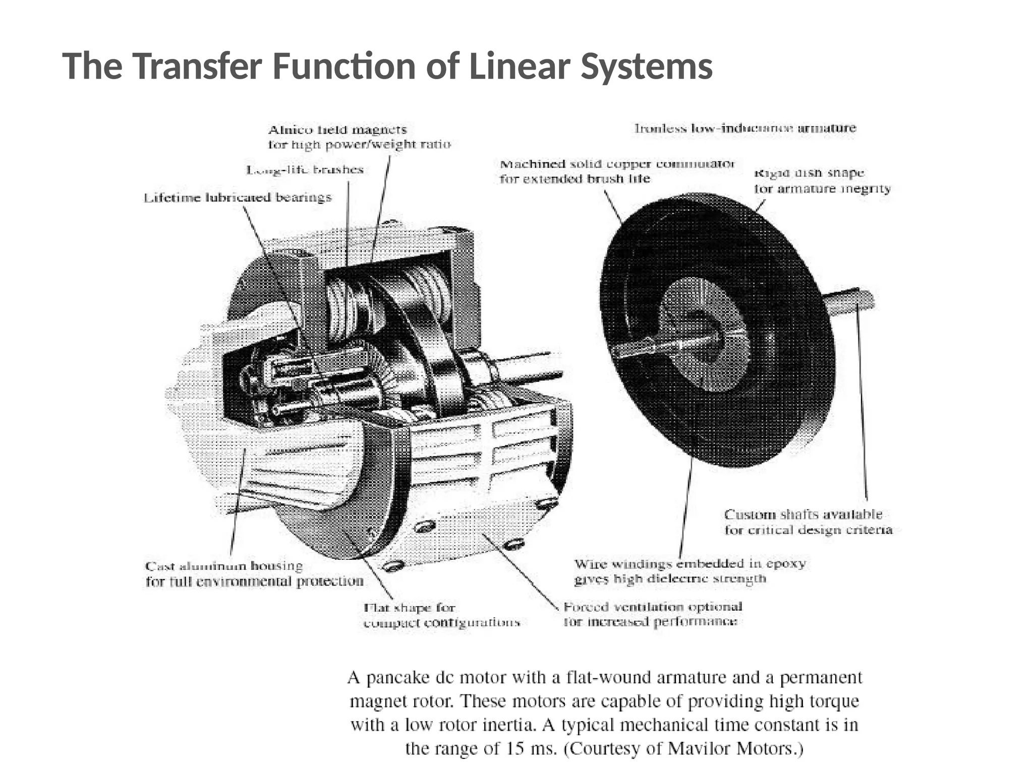
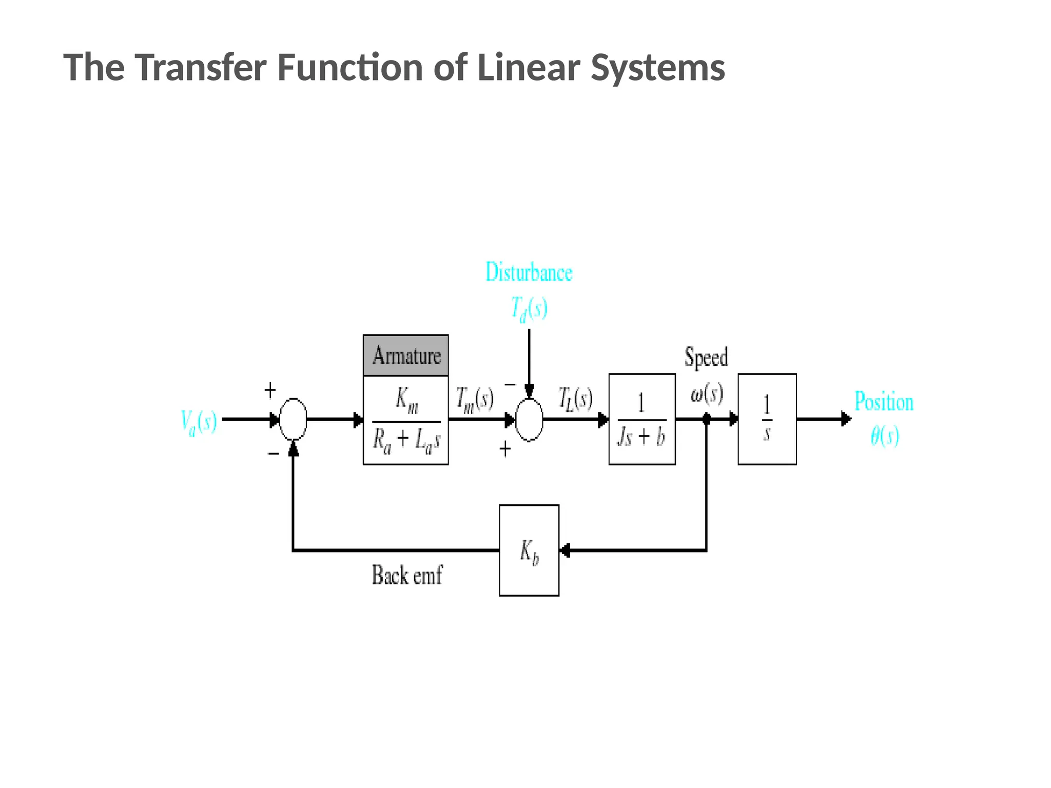
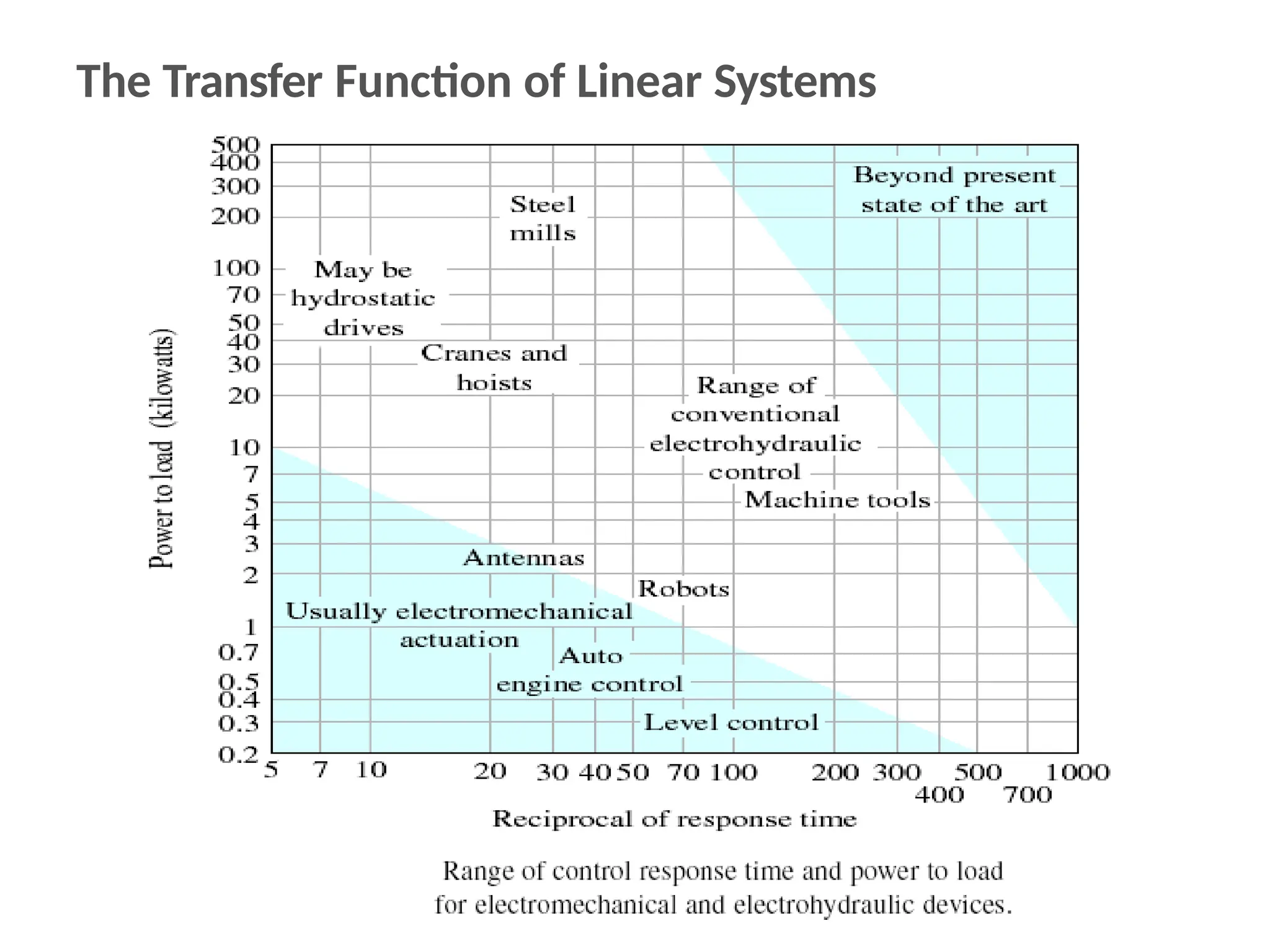
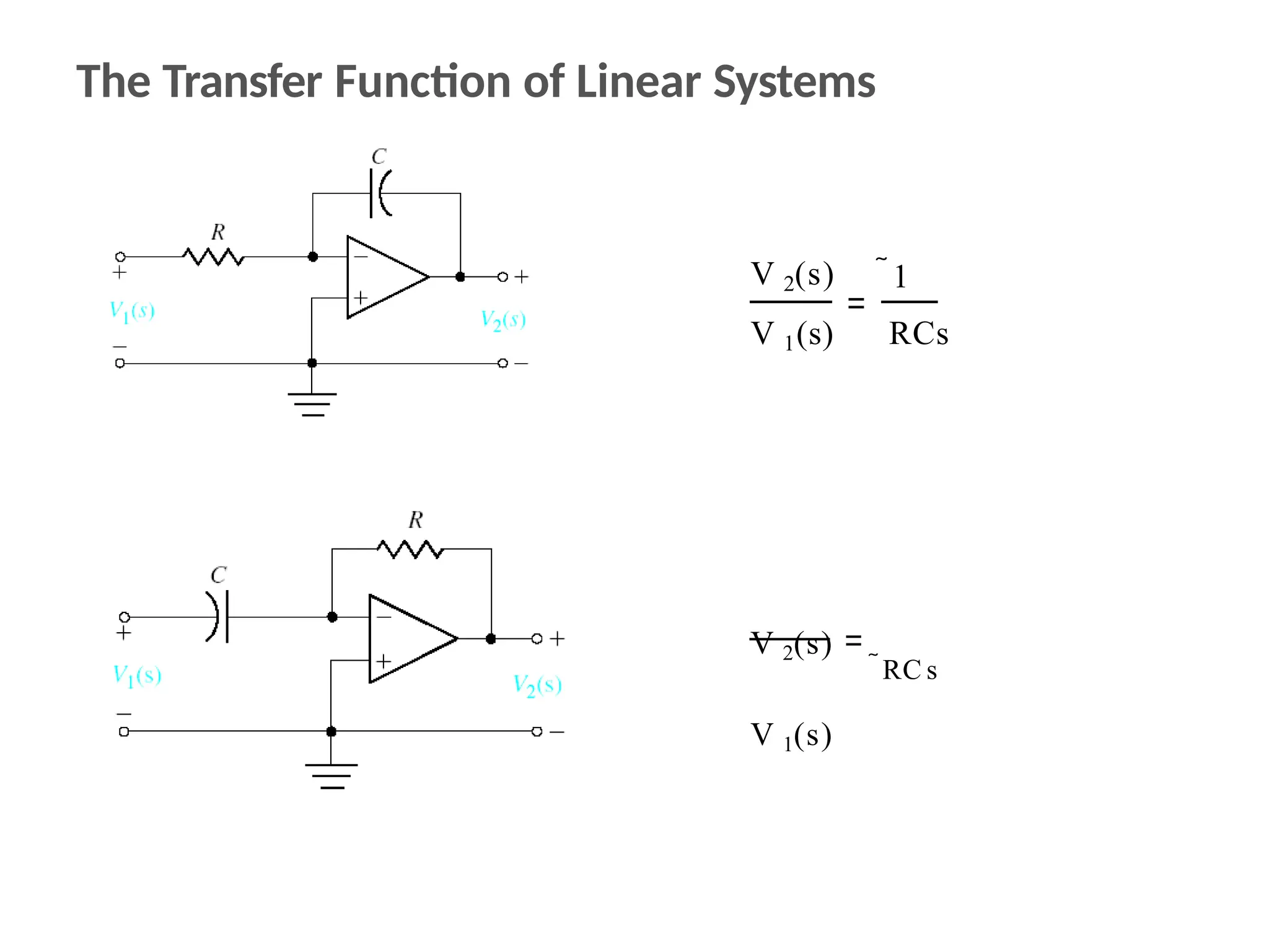
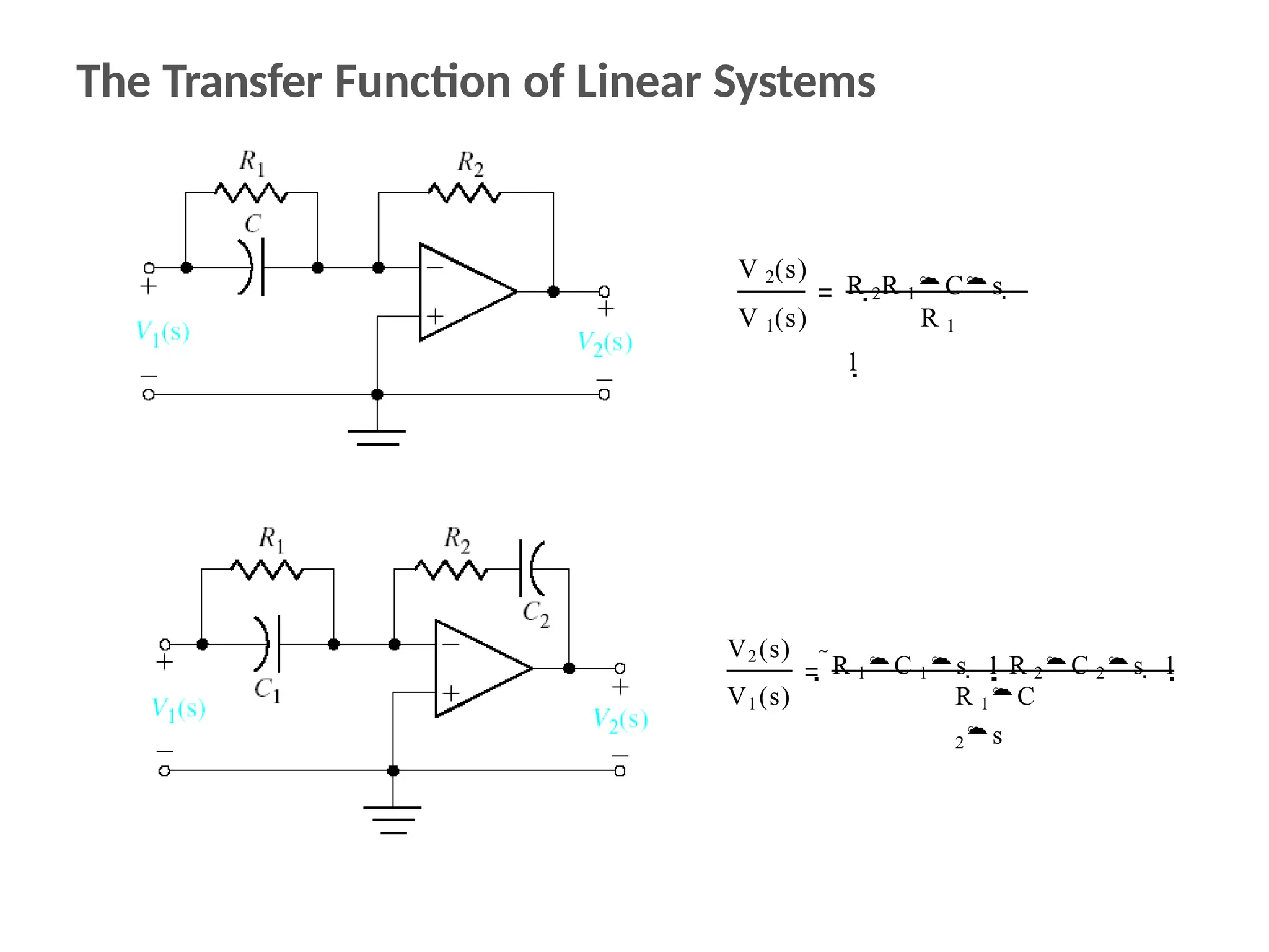
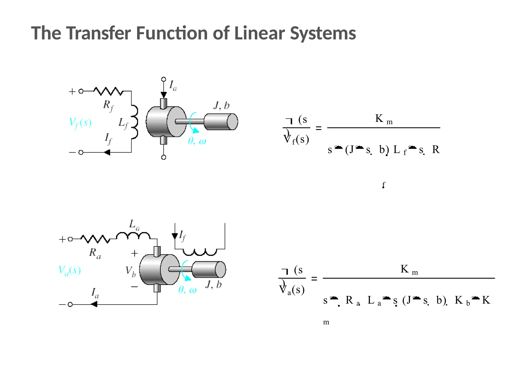
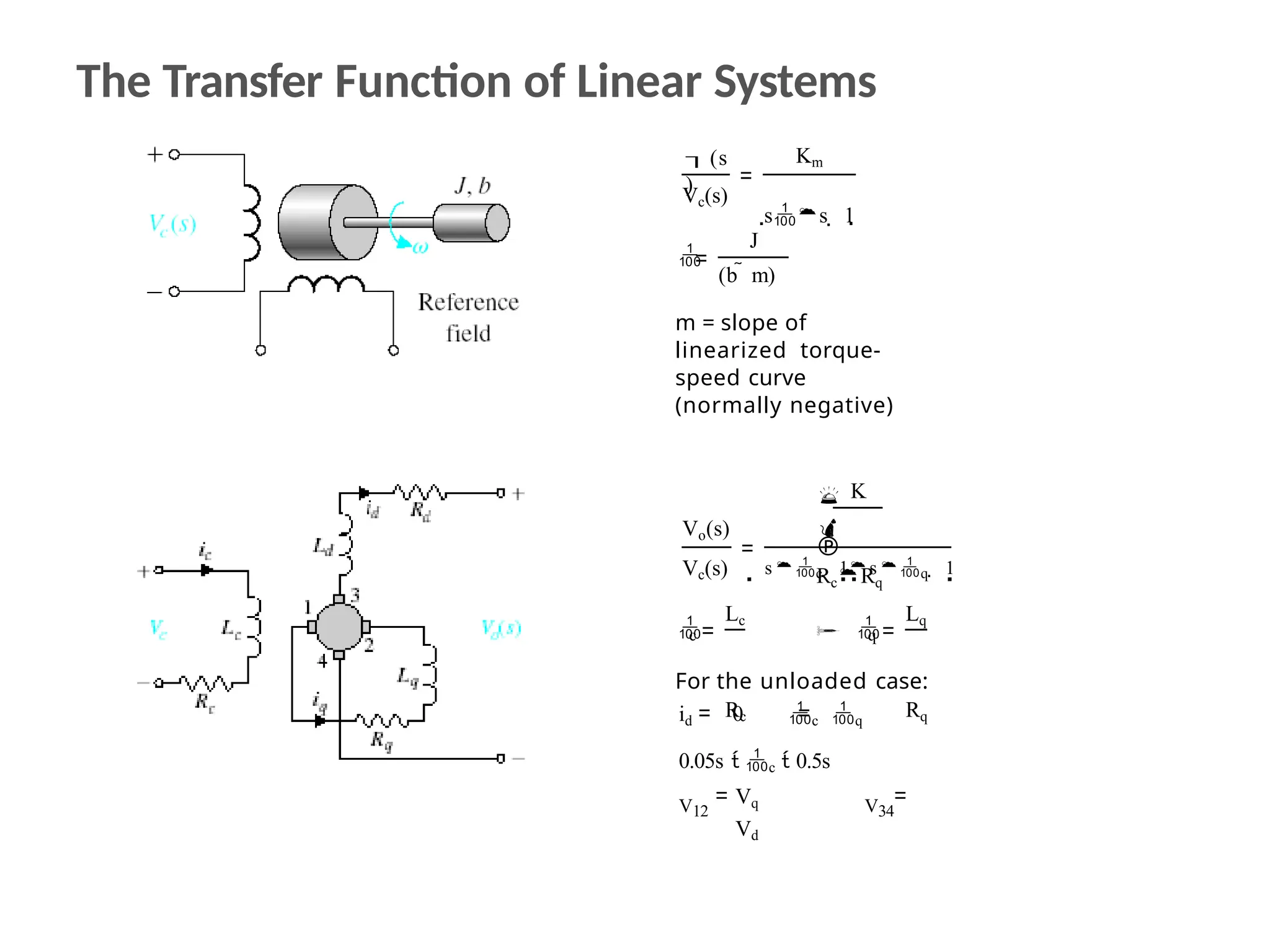
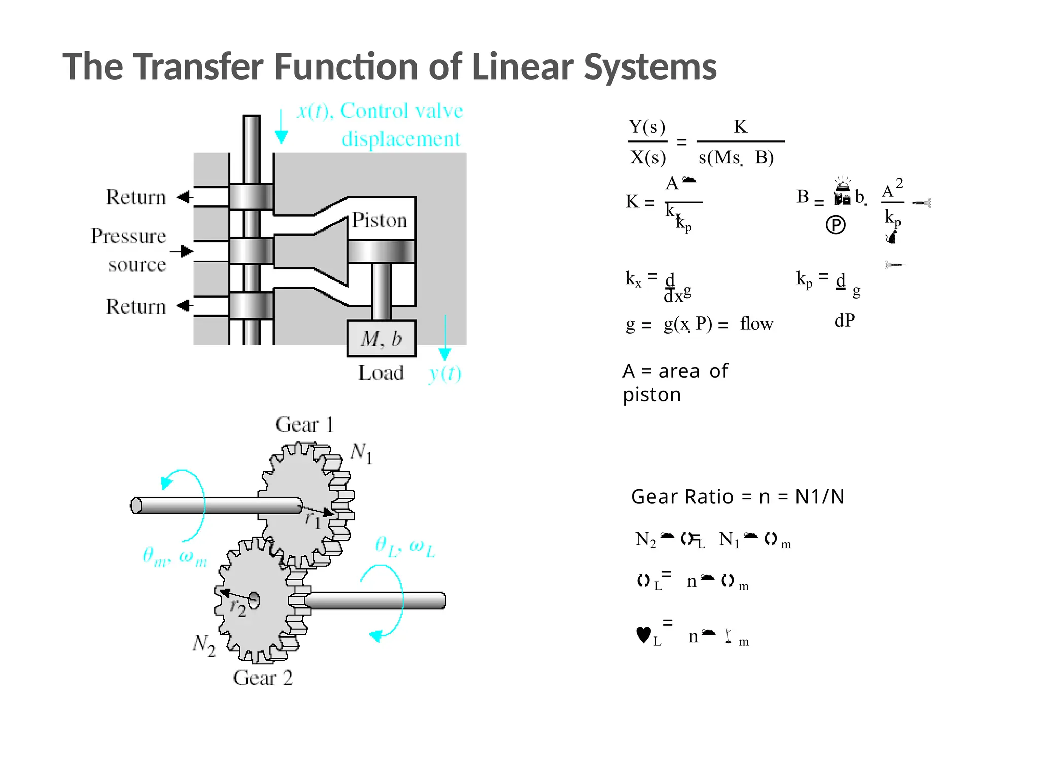
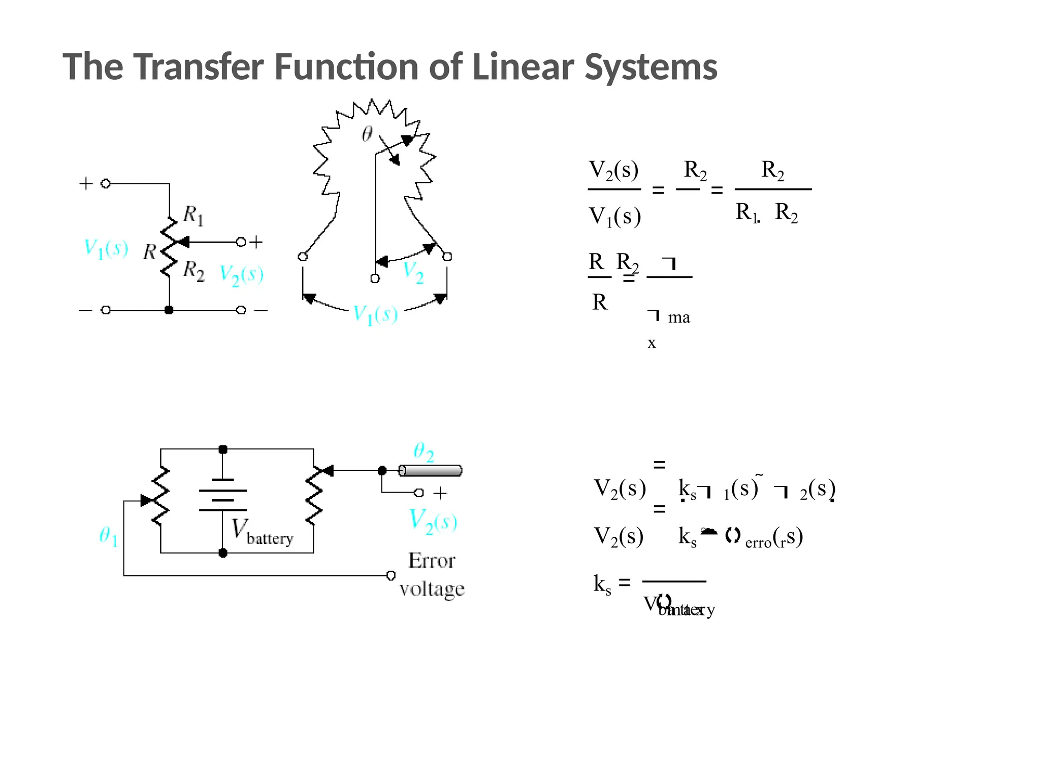
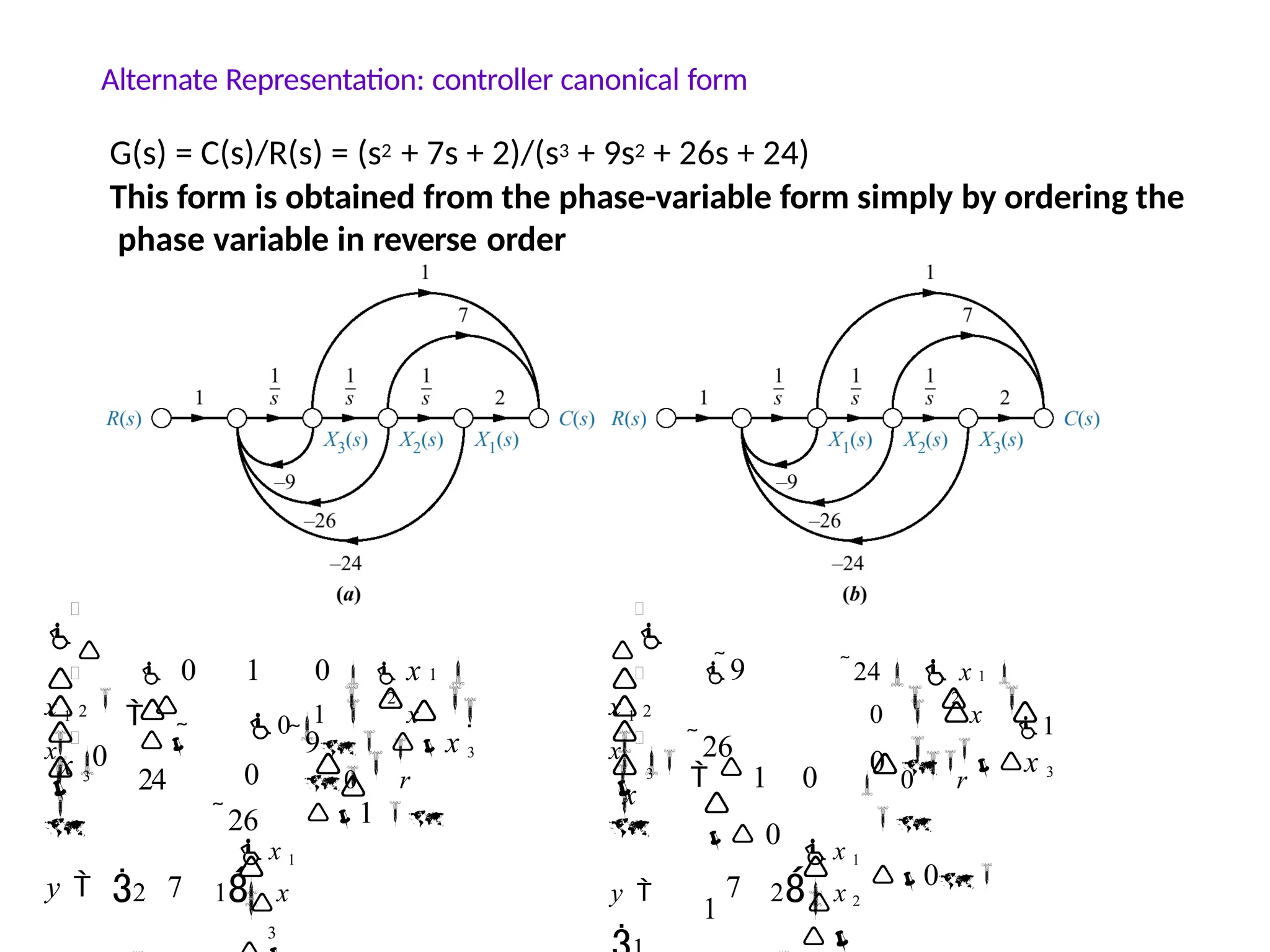
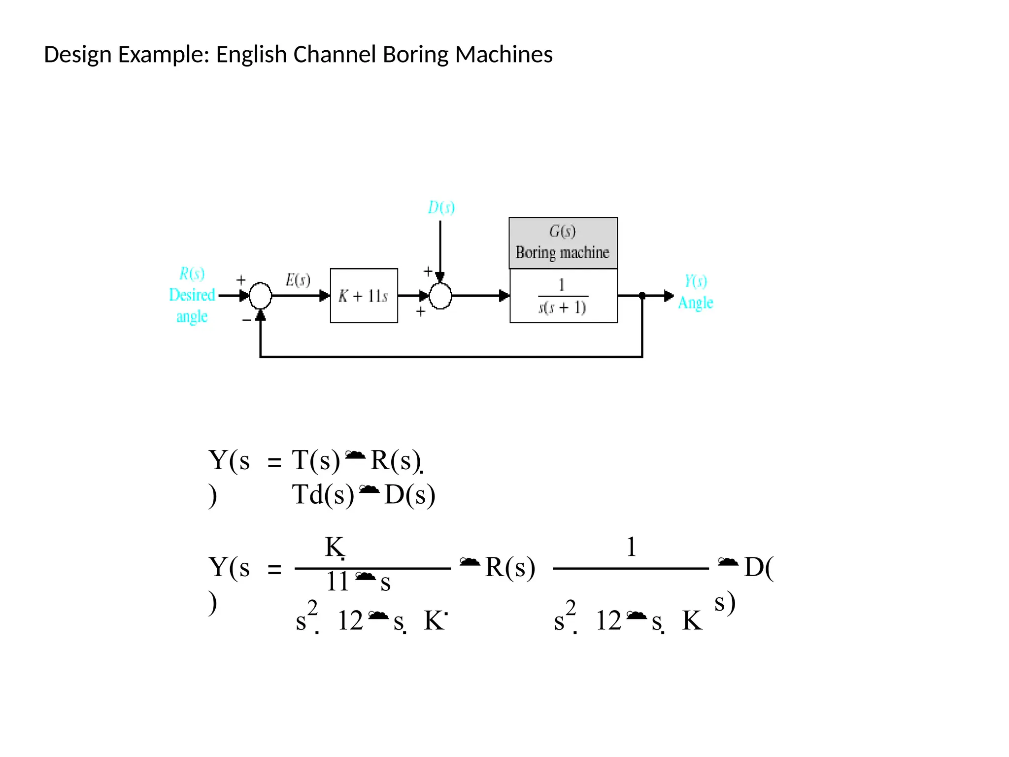
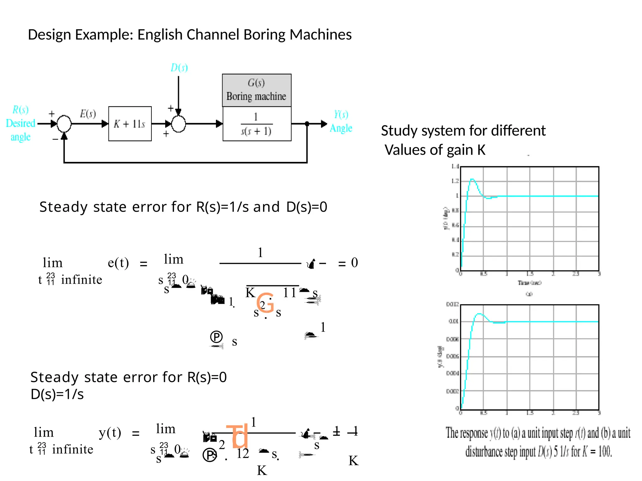
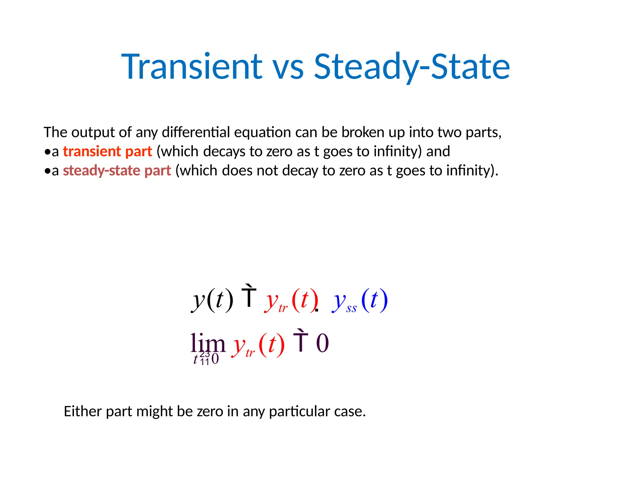
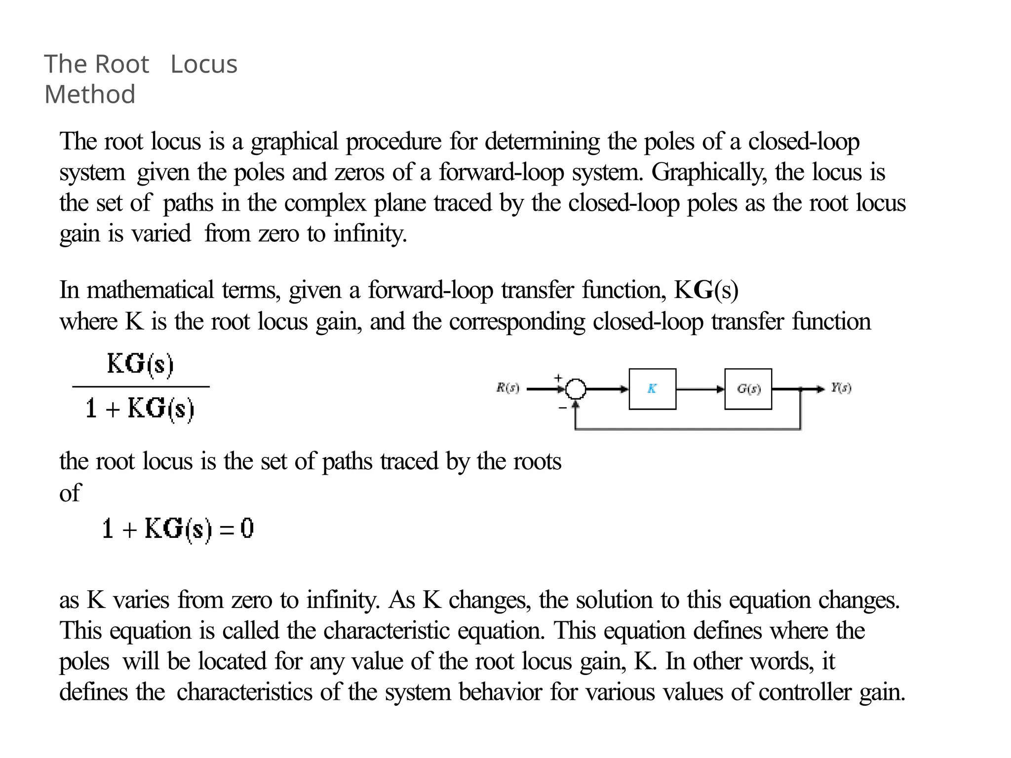
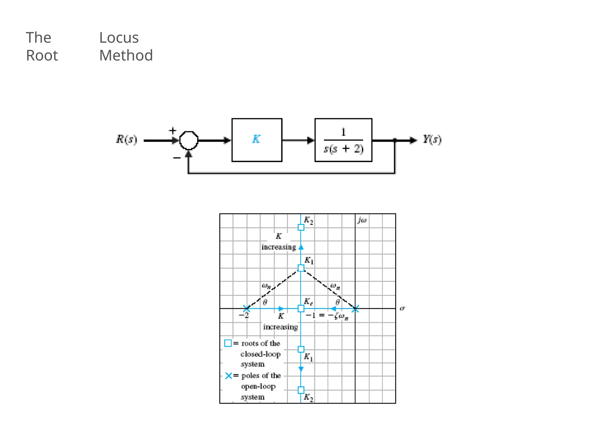
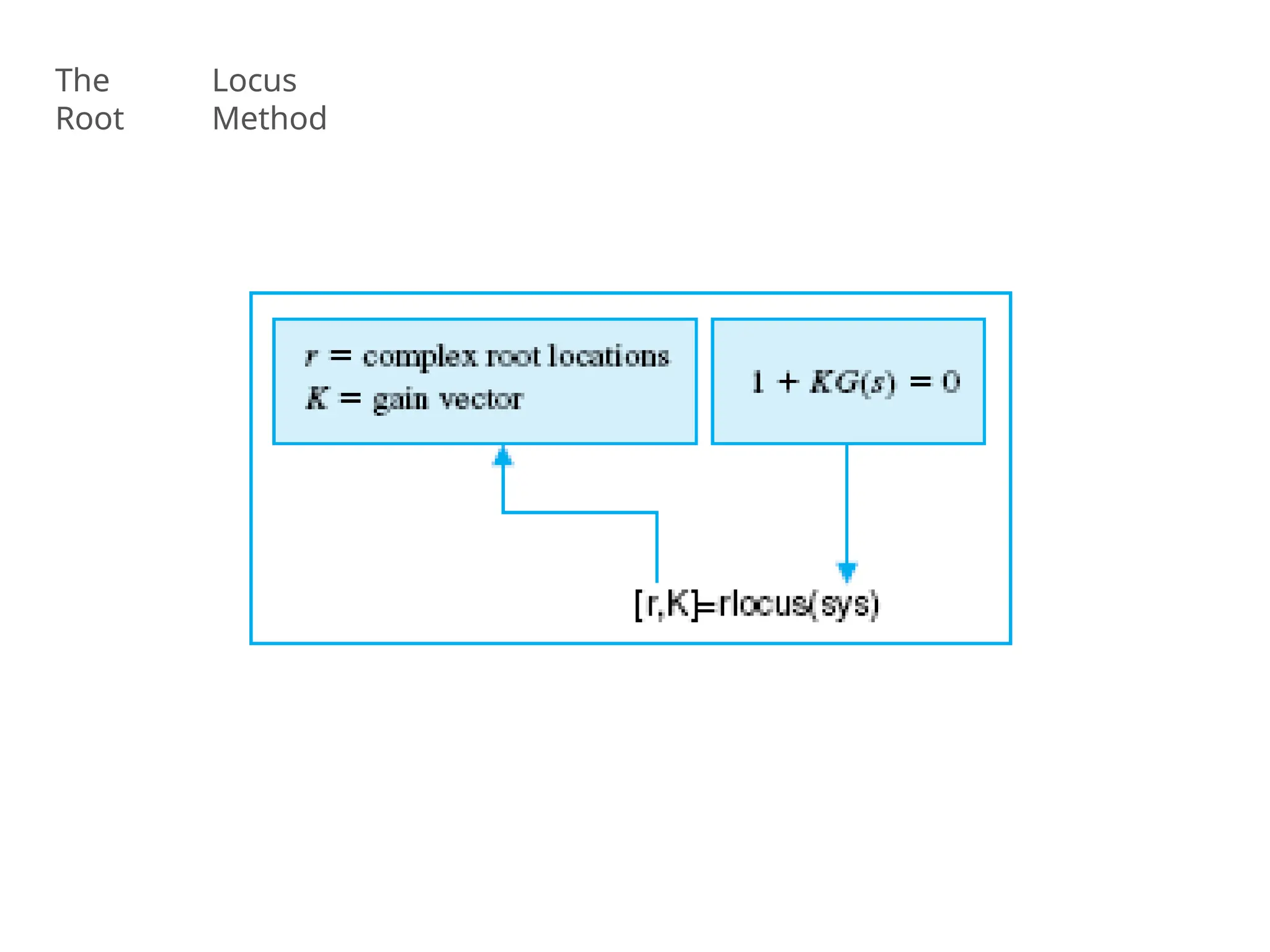
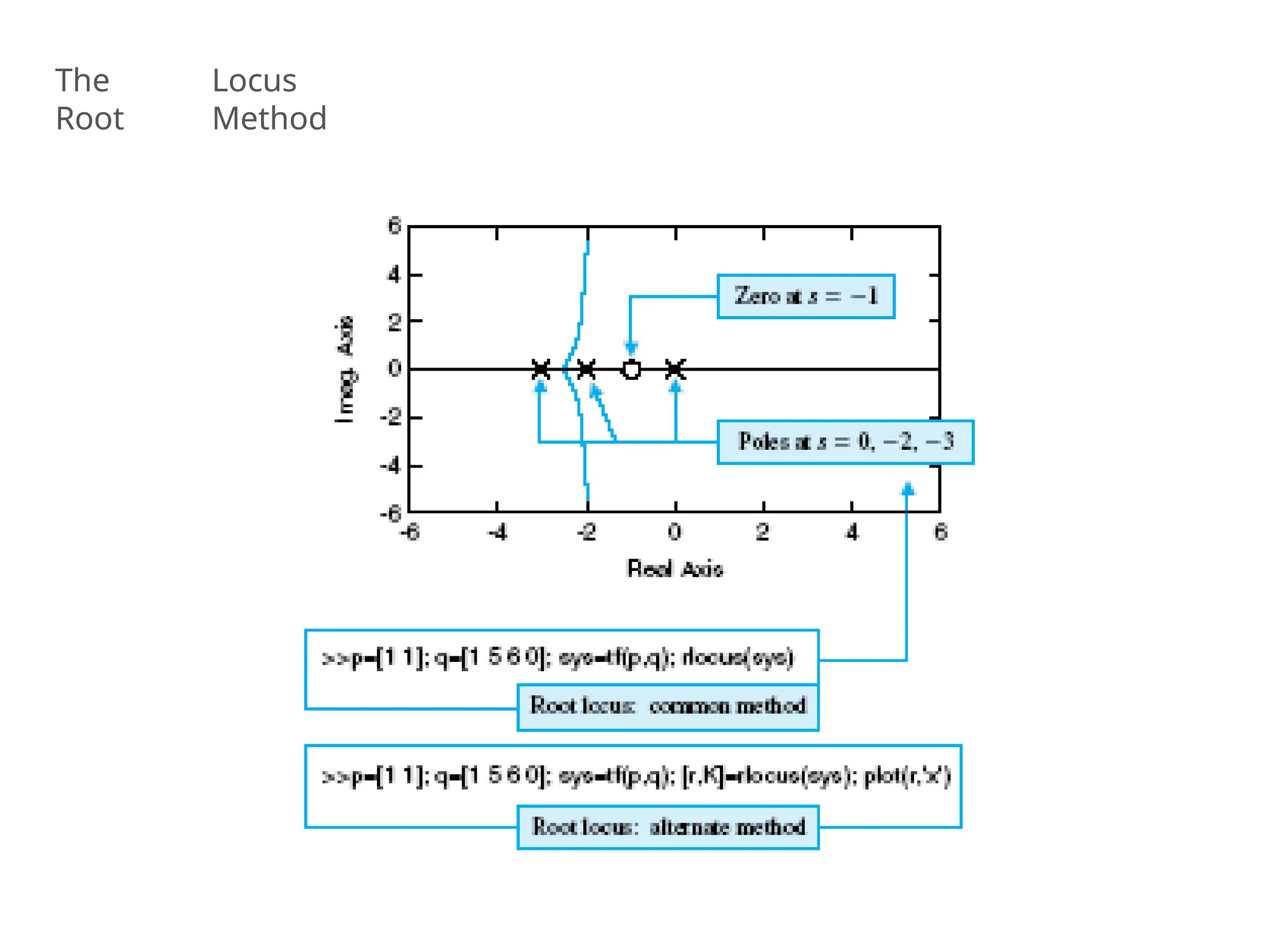
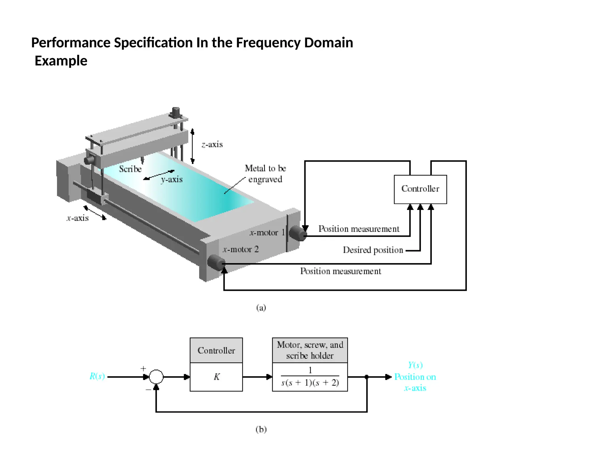
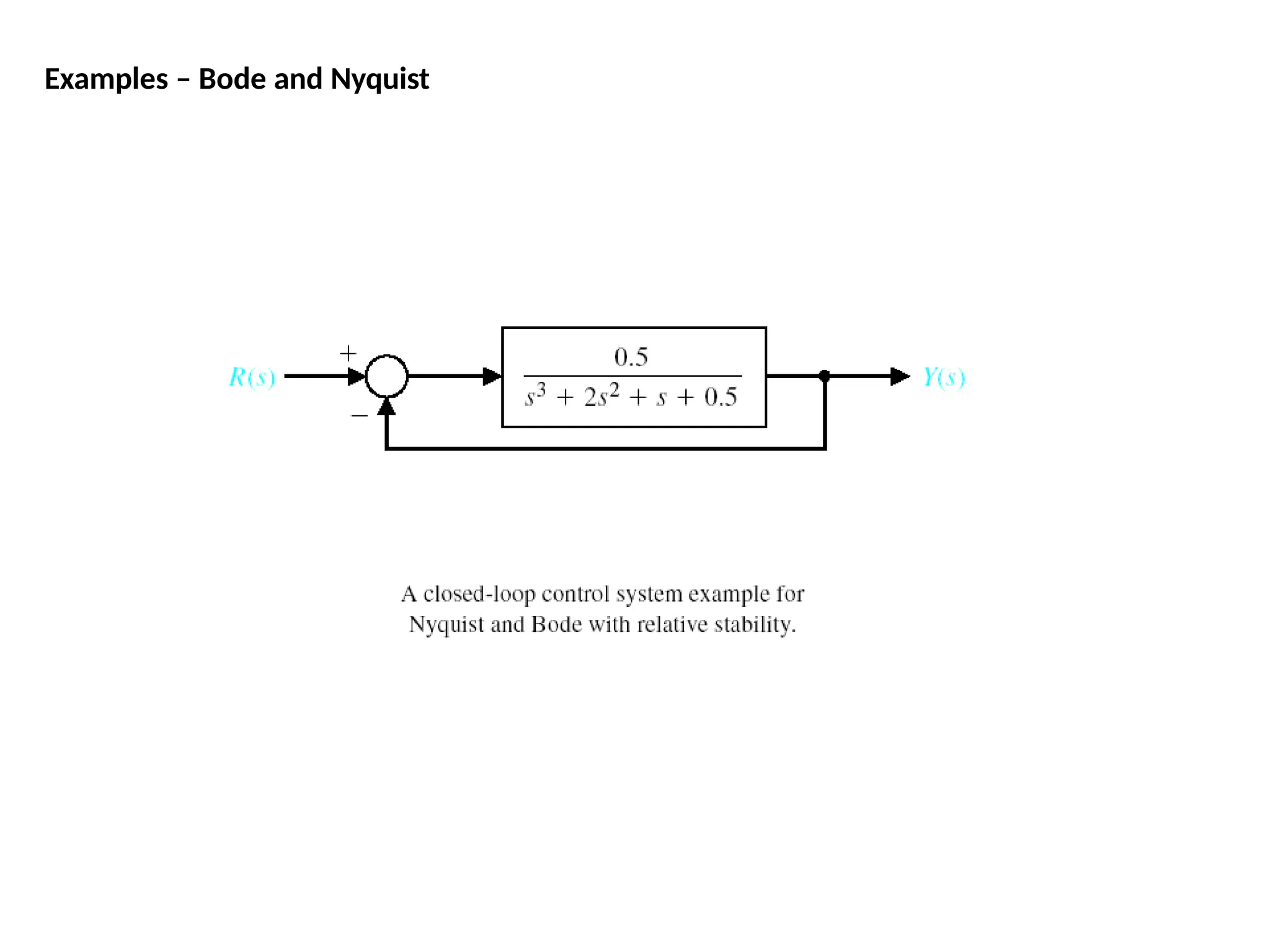
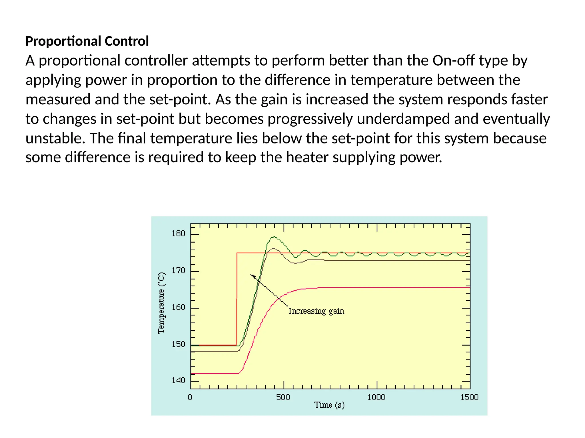
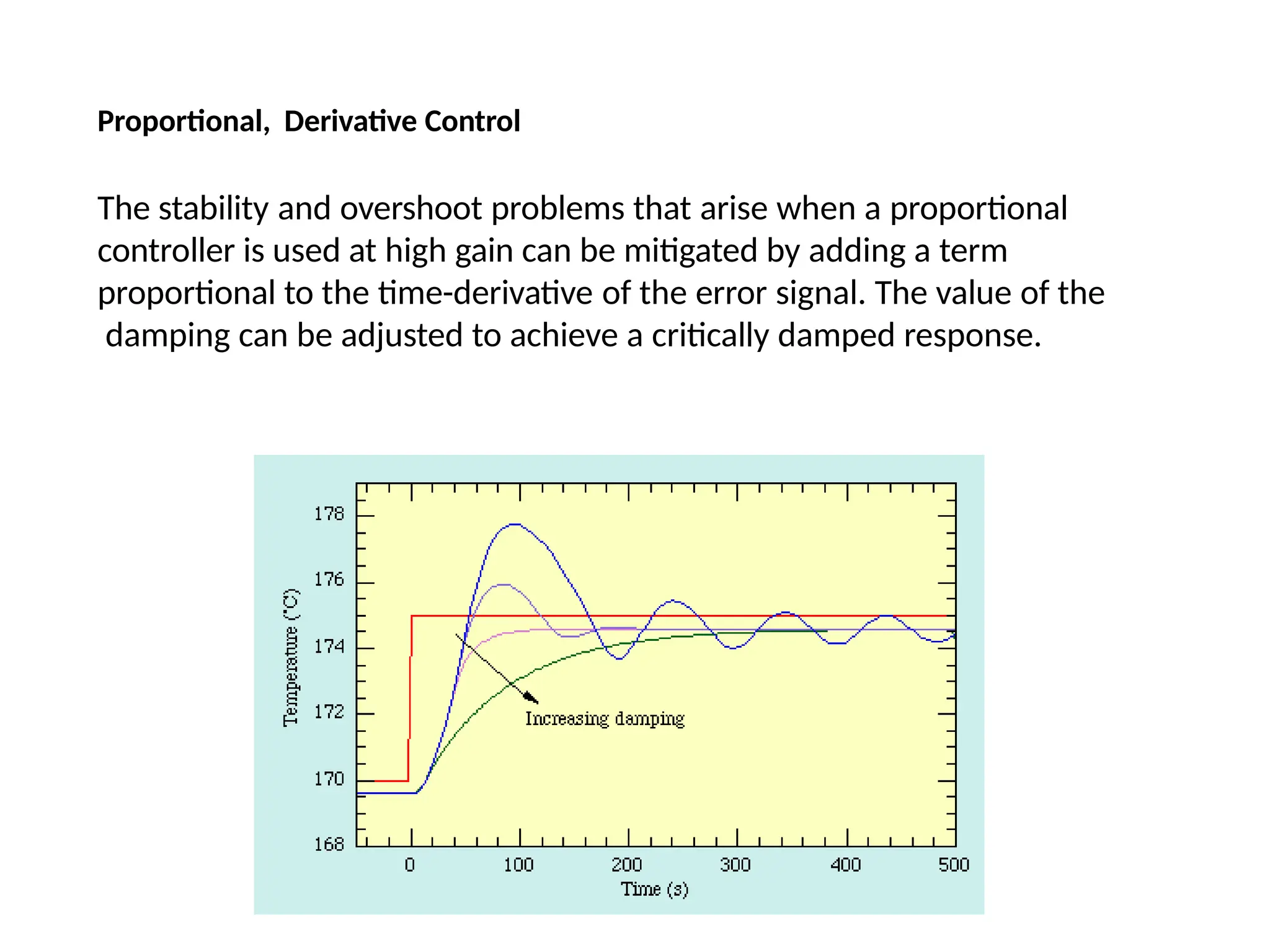
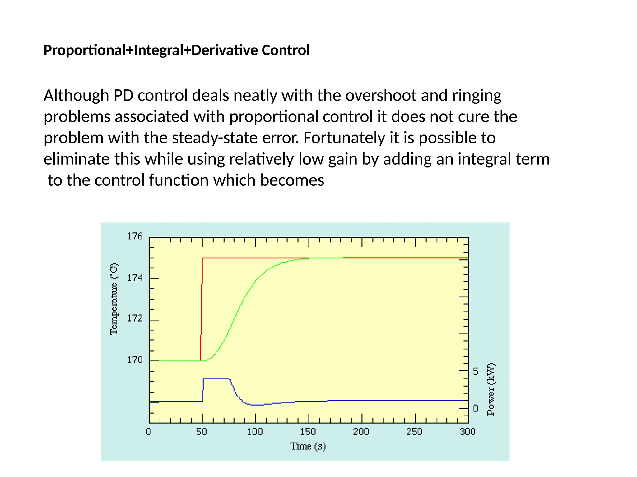
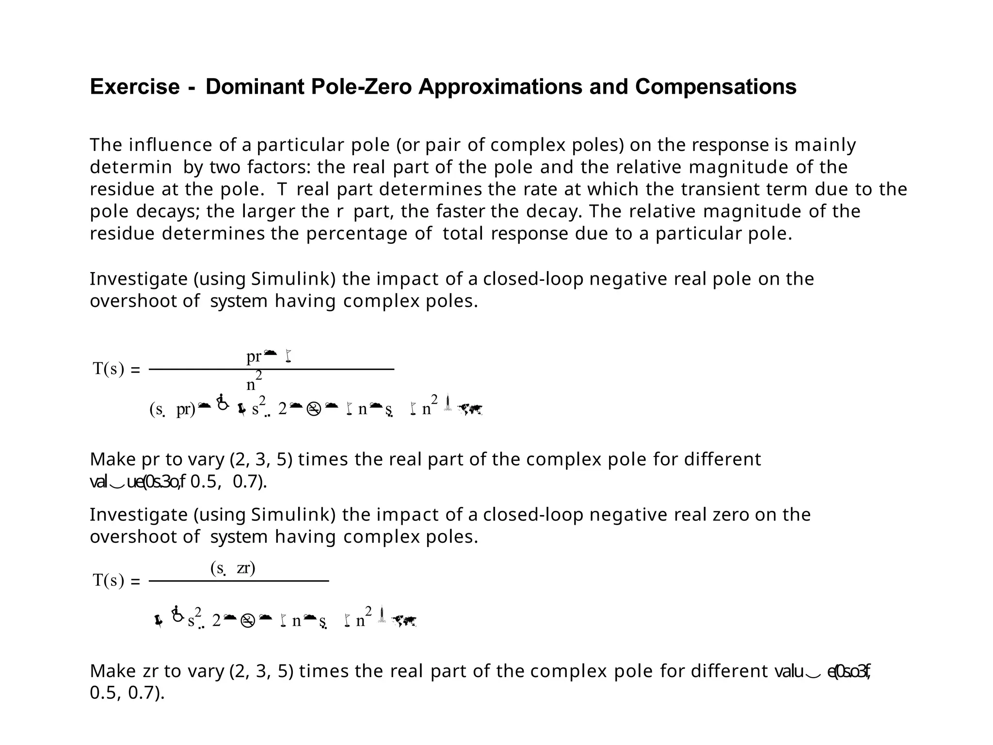
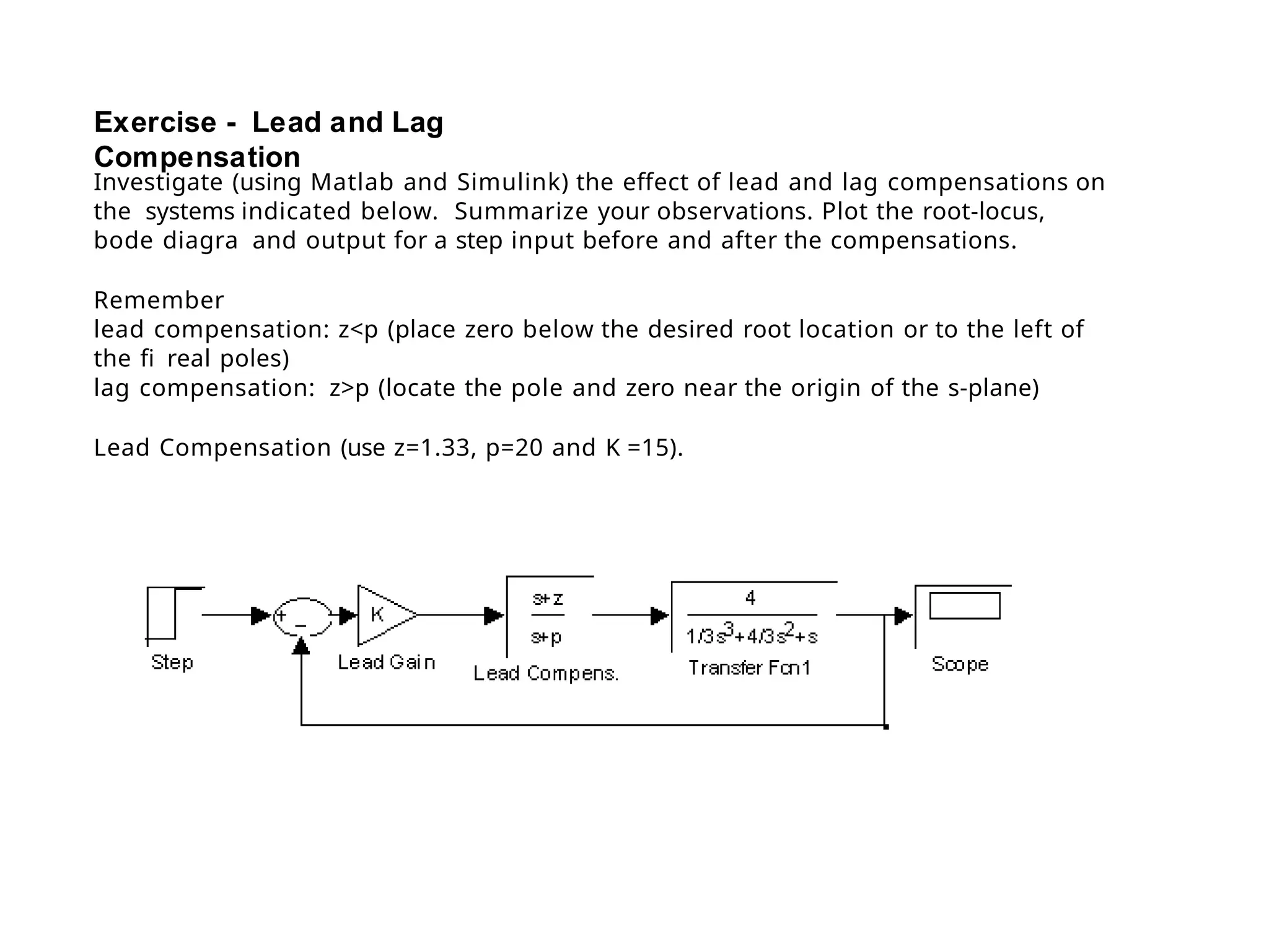
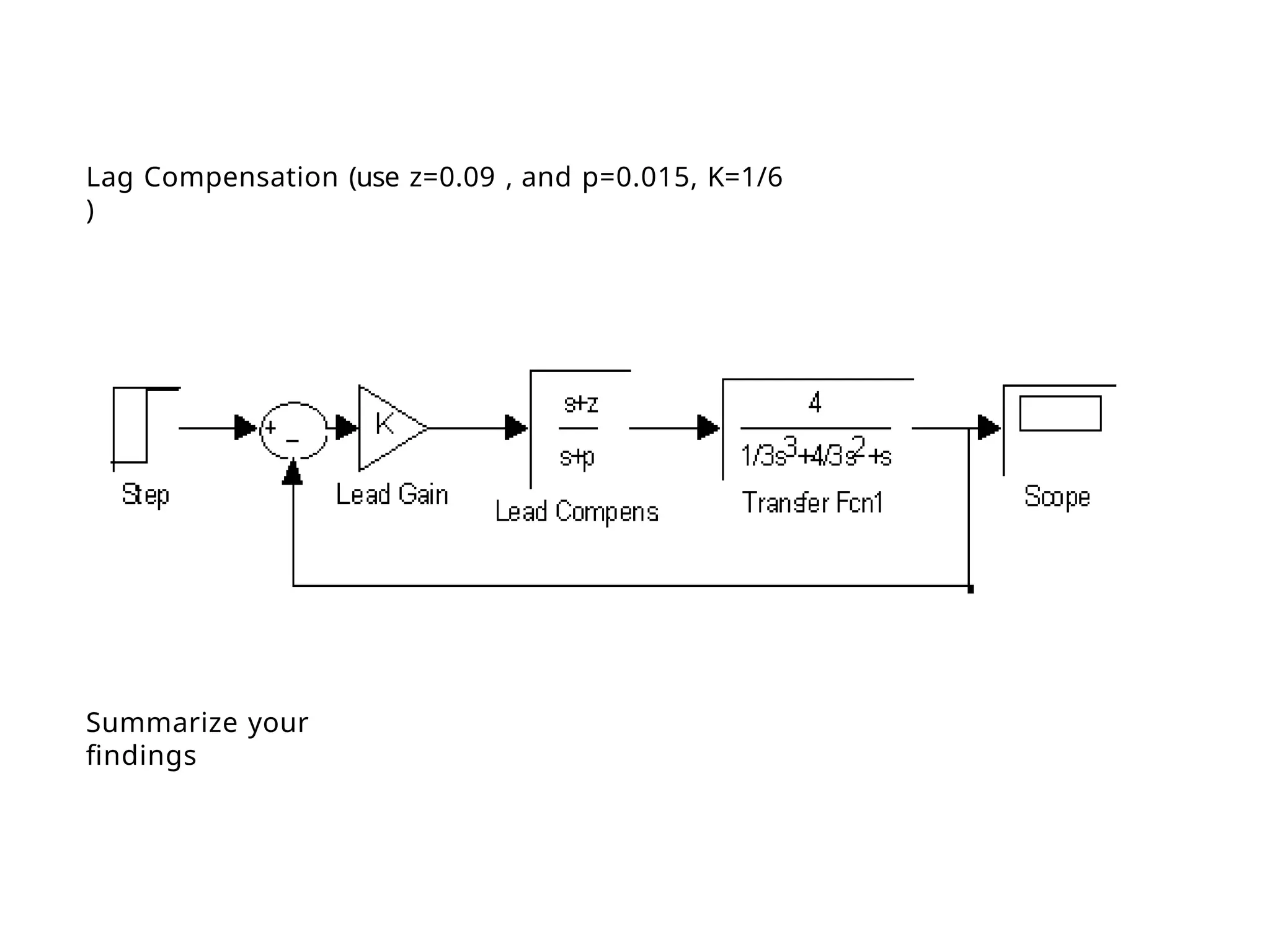
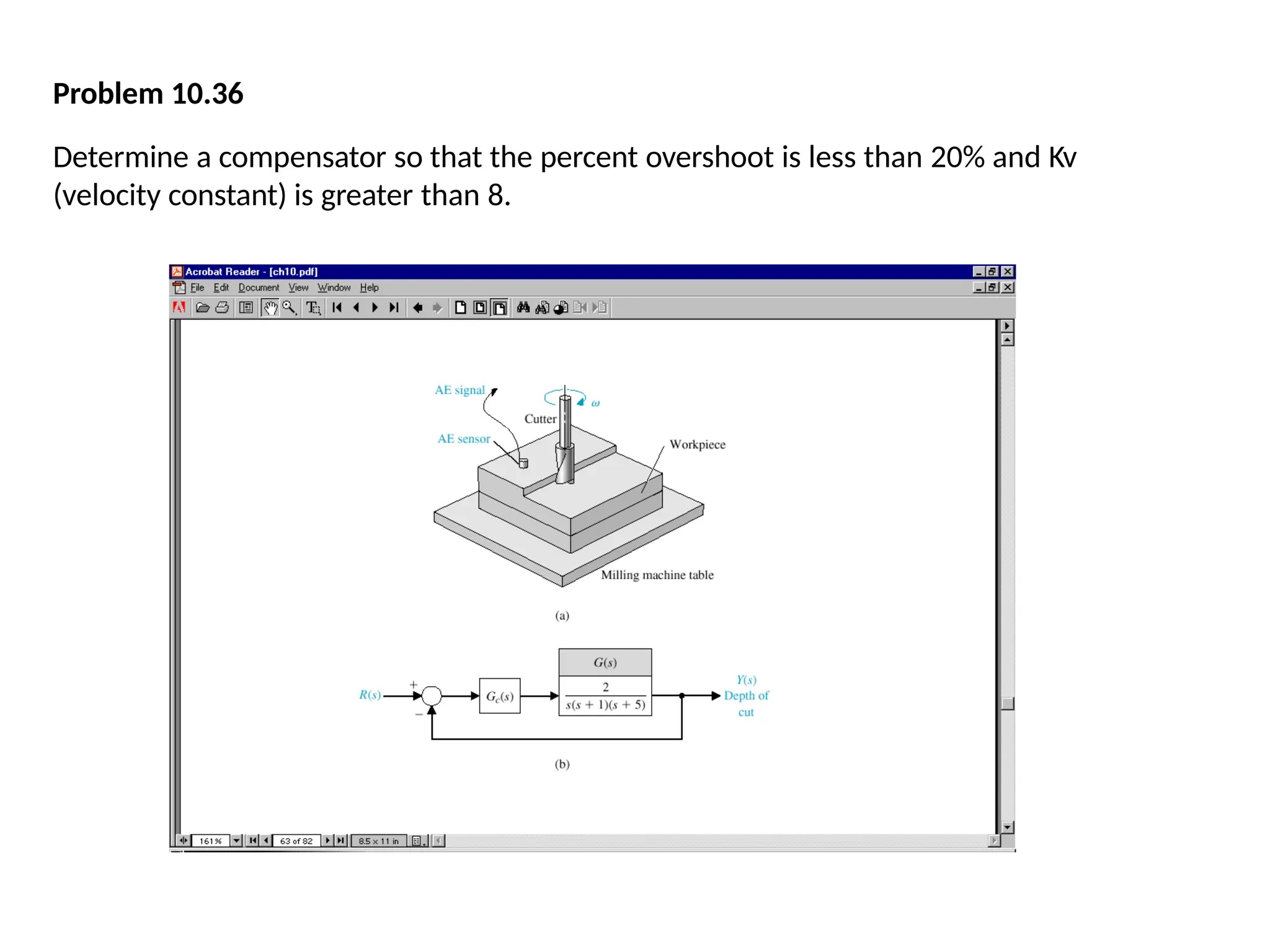
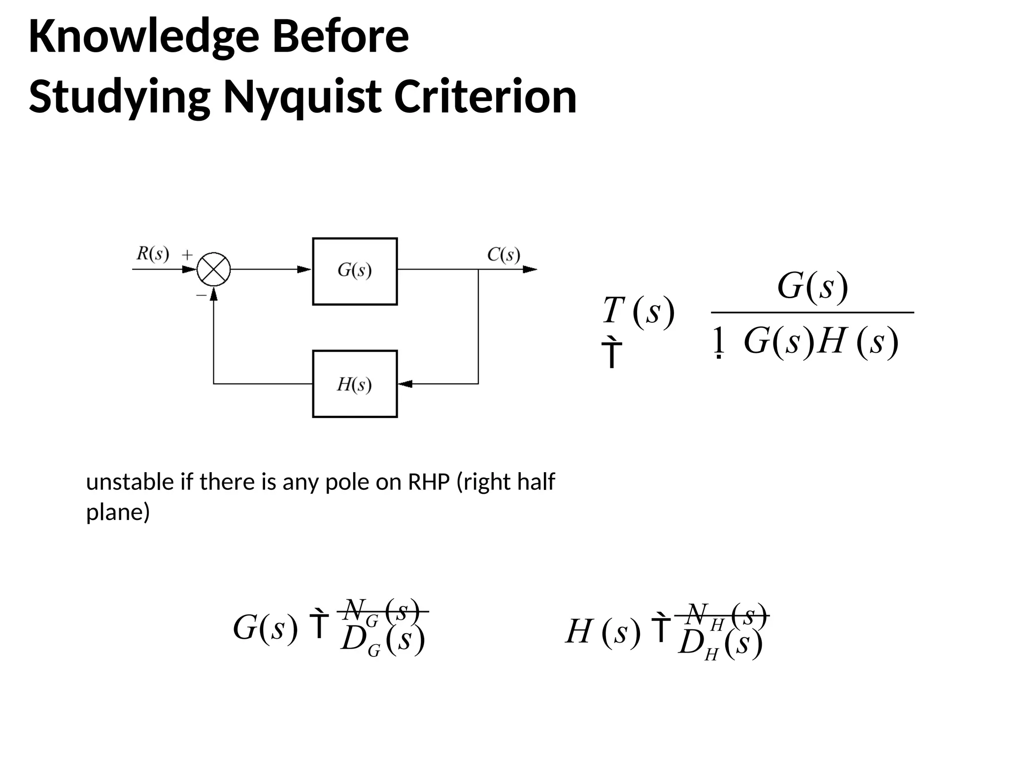
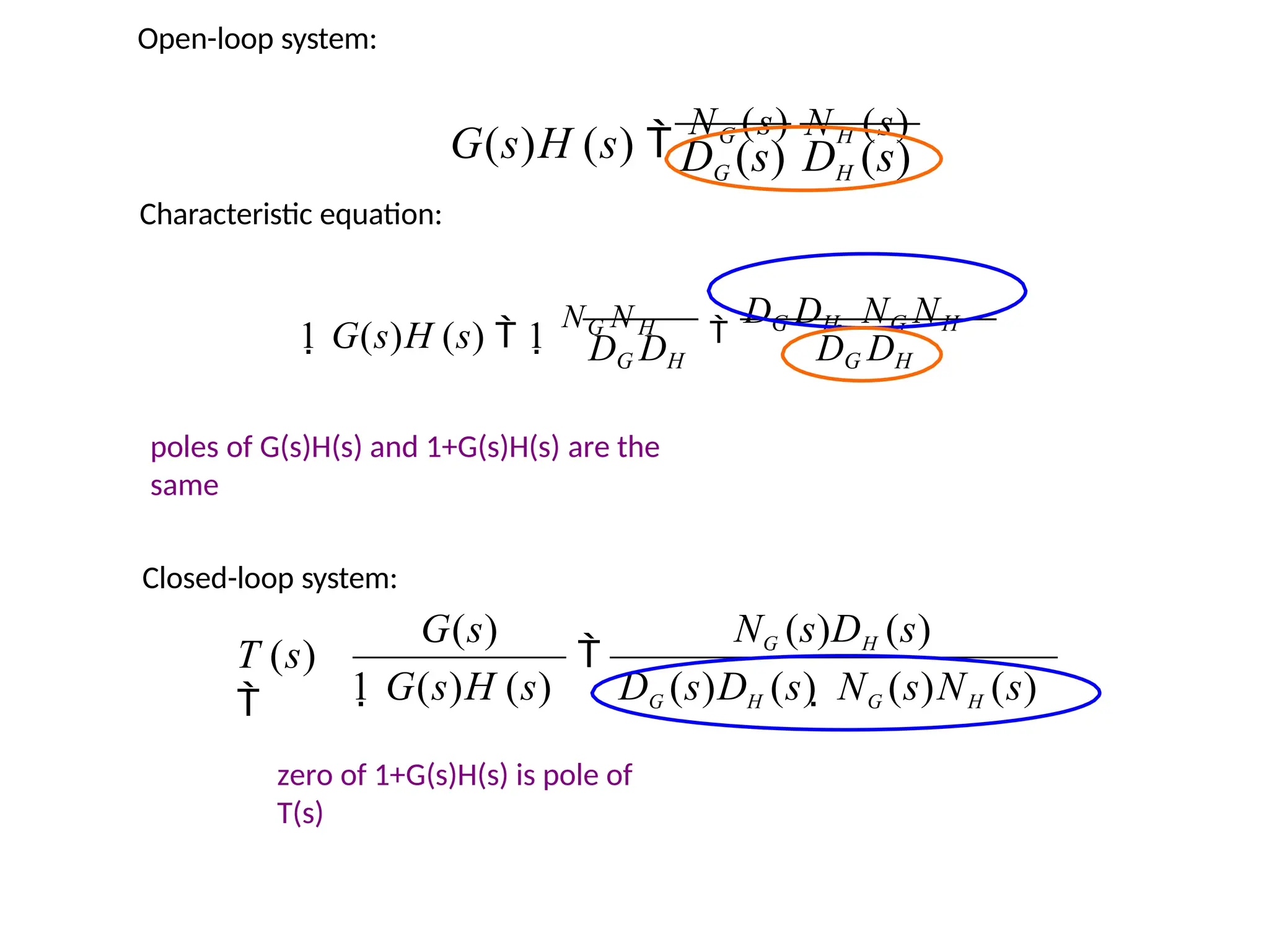
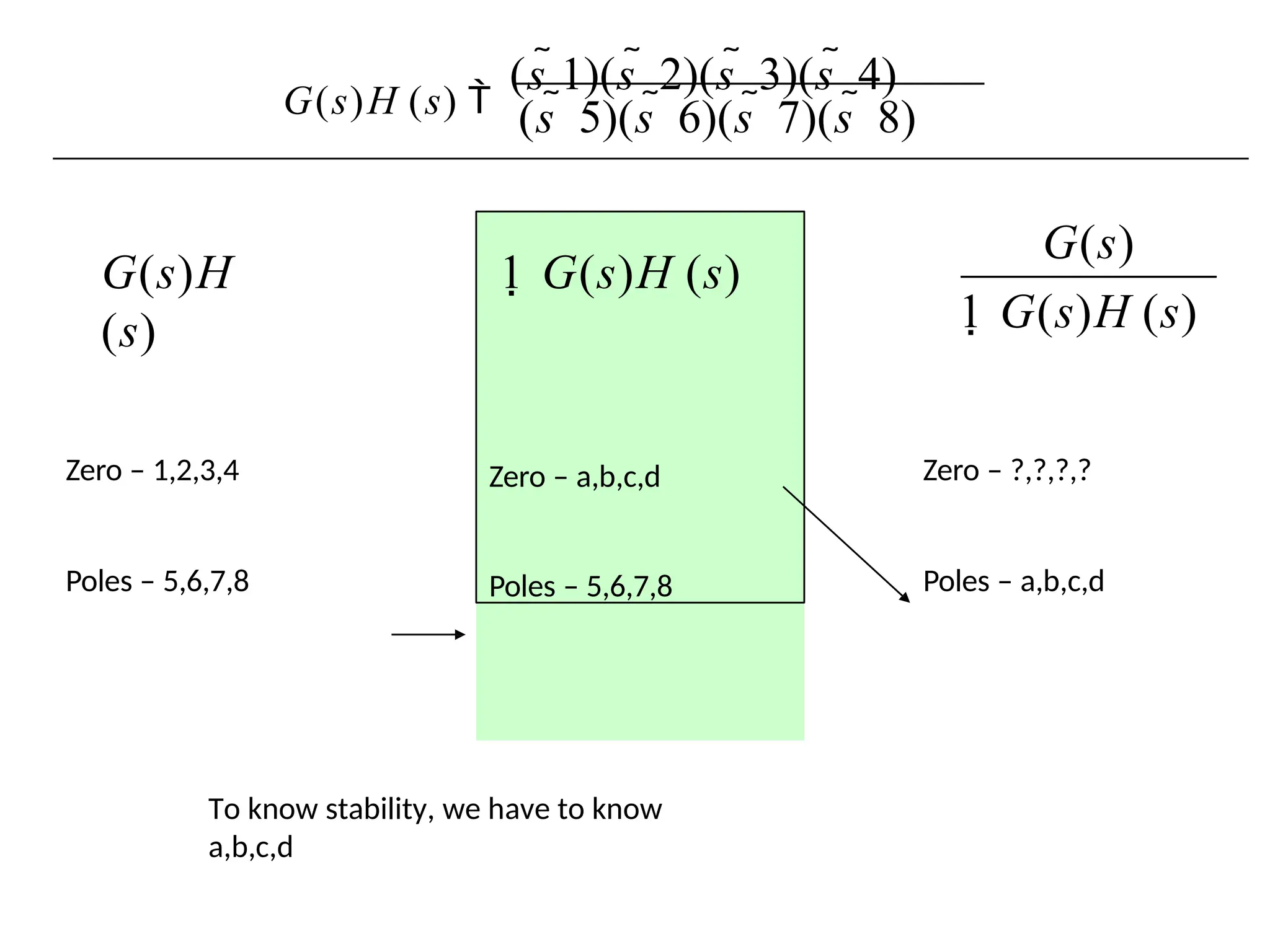
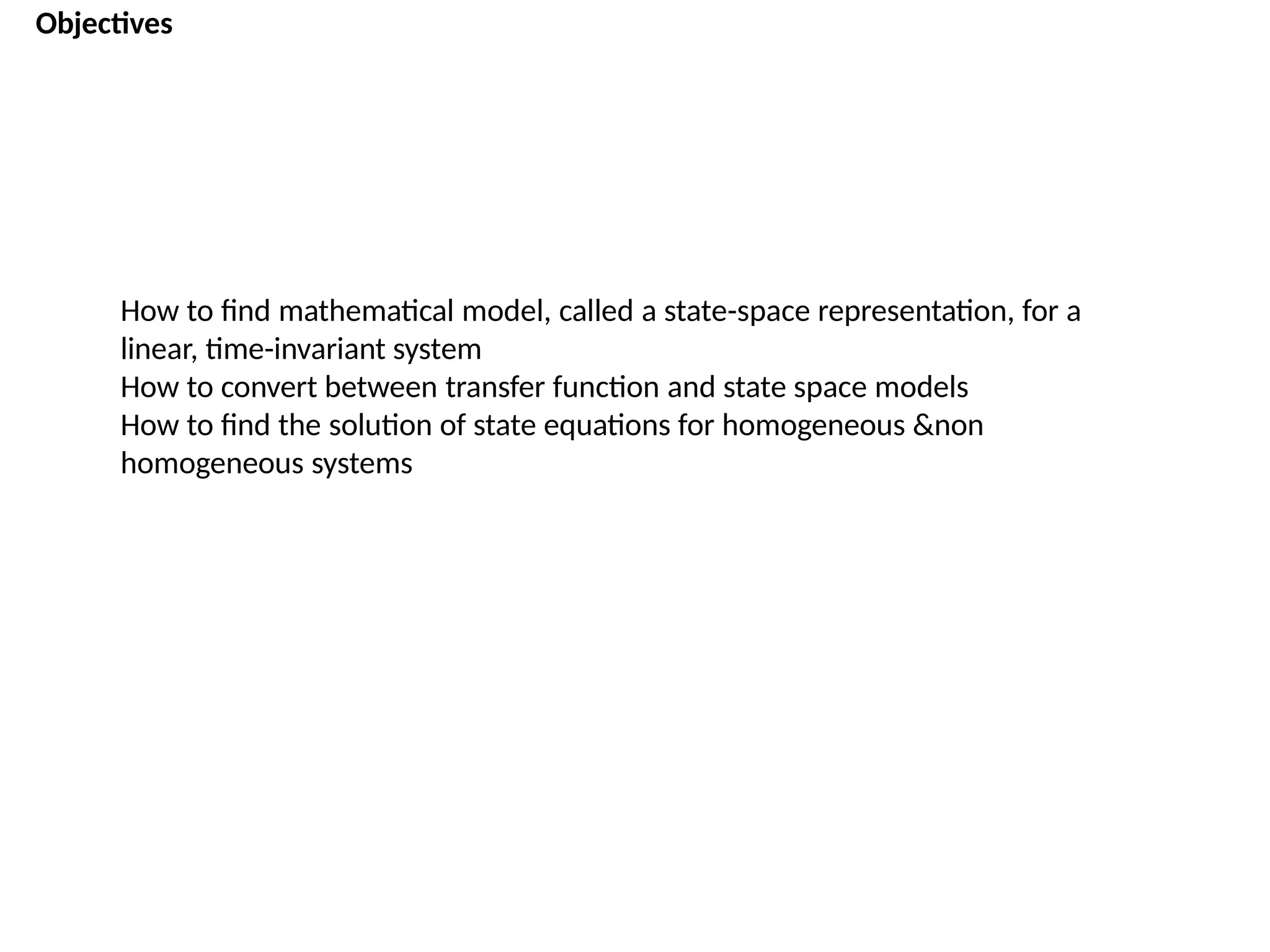
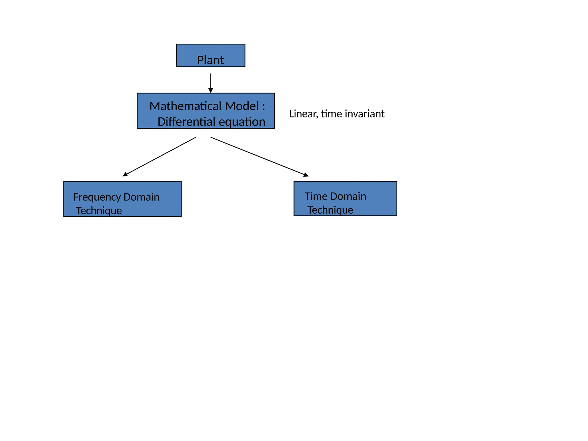
The document discusses the design and analysis of dynamic control systems using mathematical models and differential equations across various systems, including mechanical, hydraulic, and electrical. It emphasizes the use of Laplace transform methods for linearization and obtaining transfer functions, along with practical examples and techniques for solving complex equations. Additionally, it introduces electric ship concepts, highlighting their advantages in military applications through integrated power systems that enhance capabilities while reducing costs and maintenance.

![The Laplace Transform
Determine the Lap lace transform for the
functions
a) f1(t)
1
fo
r
t
0
0
dt
s
t
F1(s)
e
=
1
(st)
e s
1
s
b) f2(t)
e
(at)
F2(s)
0
dt
e
(at)
(st)
e
=
1
s 1
e
[(sa)t] 2
F (s)
1
s a](https://image.slidesharecdn.com/pptcse1-250114082557-b9789d18/75/ppt-on-Control-system-engineering-1-pptx-32-2048.jpg)
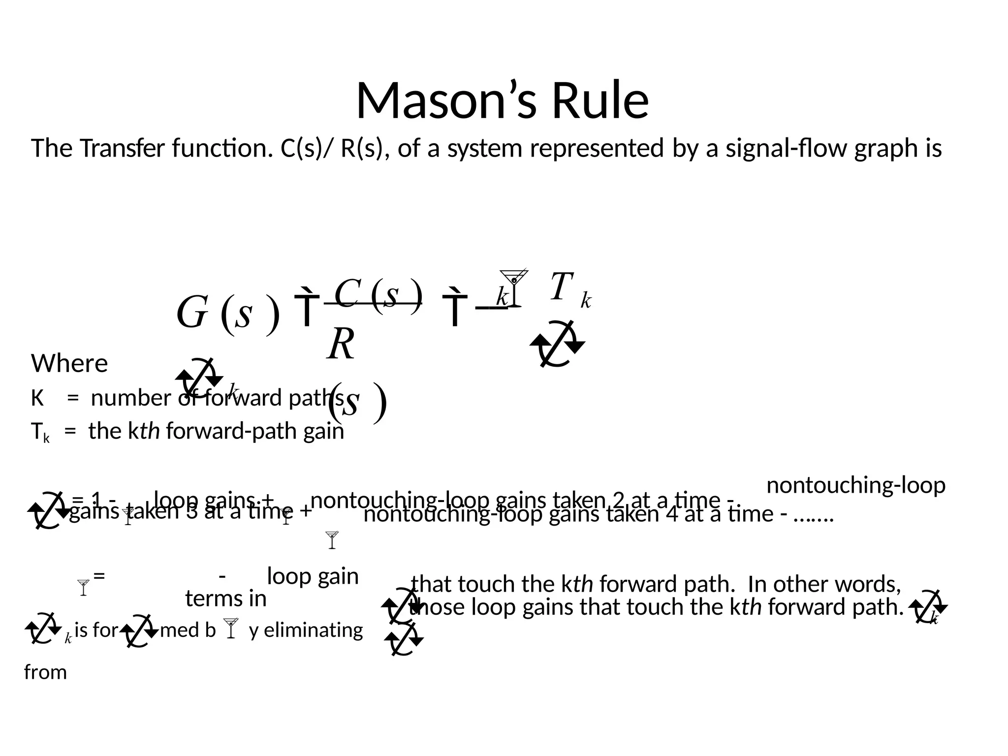
![Mason’s ƌule -
Definitions
Loop gain: The product of branch gains found by traversing a path that starts at a node and ends at the
same node, following the direction of the signal flow, without passing through any other node more than
once. G2(s)H2(s), G4(s)H2(s), G4(s)G5(s)H3(s), G4(s)G6(s)H3(s)
Forward-path gain: The product of gains found by traversing a path from input node to output node in
the direction of signal flow. G1(s)G2(s)G3(s)G4(s)G5(s)G7(s), G1(s)G2(s)G3(s)G4(s)G5(s)G7(s)
Nontouching loops: loops that do not have any nodes in common. G2(s)H1(s) does not touch G4(s)H2(s),
G4(s)G5(s)H3(s), and G4(s)G6(s)H3(s)
Nontouching-loop gain: The product of loop gains from nontouching loops taken 2, 3,4, or more at a
time.
[G2(s)H1(s)][G4(s)H2(s)], [G2(s)H1(s)][G4(s)G5(s)H3(s)], [G2(s)H1(s)][G4(s)G6(s)H3(s)]](https://image.slidesharecdn.com/pptcse1-250114082557-b9789d18/75/ppt-on-Control-system-engineering-1-pptx-98-2048.jpg)
![Transfer function via Mason’s rule
Now
Problem: Find the transfer function for the signal flow graph
Solution:
forward path
G1(s)G2(s)G3(s)G4(s)G5(s)
Loop gains
G2(s)H1(s), G4(s)H2(s), G7(s)H4(s),
G2(s)G3(s)G4(s)G5(s)G6(s)G7(s)G8(s)
Nontouching loops
2at a time
G2(s)H1(s)G4(s)H2(s)
G2(s)H1(s)G7(s)H4(s)
G4(s)H2(s)G7(s)H4(s)
3at a time
G2(s)H1(s)G4(s)H2(s)
G7(s)H4(s)
= 1-
[G2(s)H1(s)
+G4(s)H2(s)
+G7(s)H4(s)+
[G1(s)G2(s)G3(s)G4(s)G5(s)][1-G7(s)H4(s)]
G (s )
T11 ](https://image.slidesharecdn.com/pptcse1-250114082557-b9789d18/75/ppt-on-Control-system-engineering-1-pptx-100-2048.jpg)
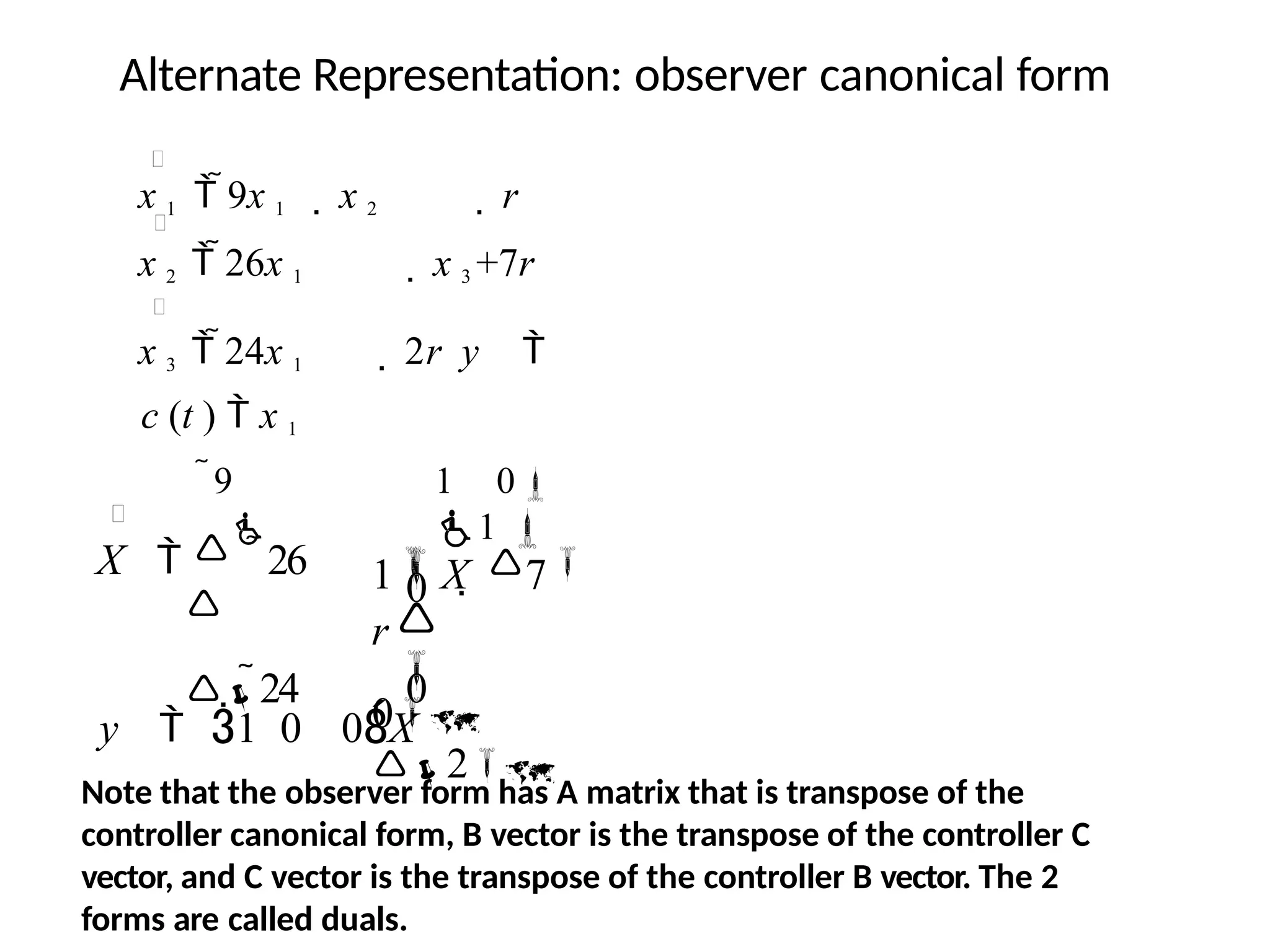
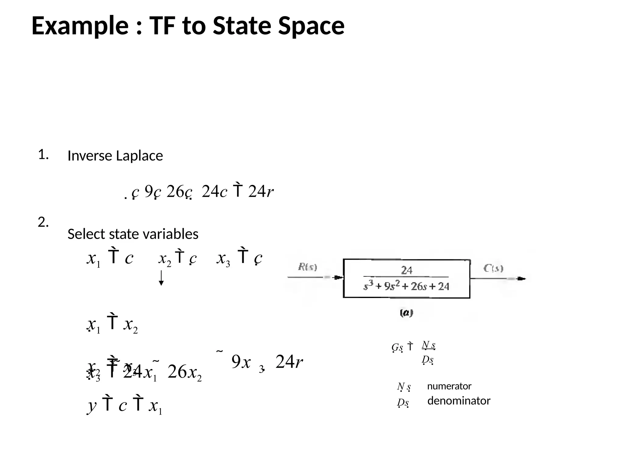
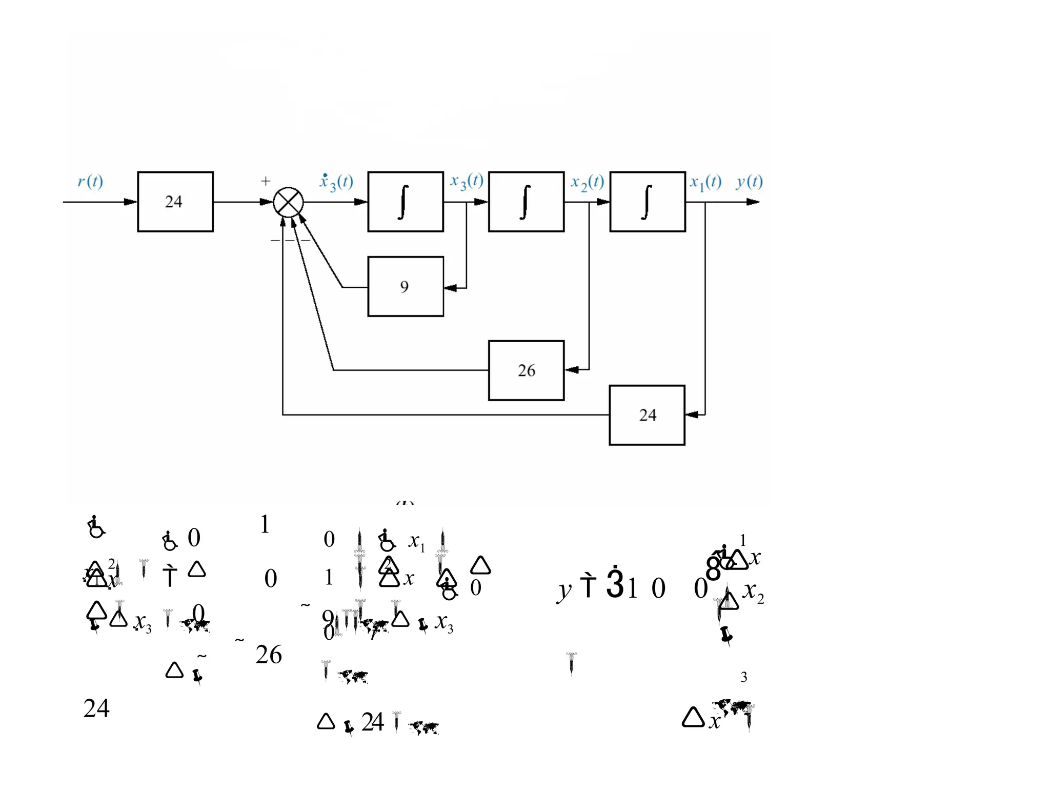
![Alternate Representation: observer canonical form
Observer canonical form so named for its use in the design of observers
G(s) = C(s)/R(s) = (s2 + 7s + 2)/(s3 + 9s2 + 26s + 24)
= (1/s+7/s2 +2/s3 )/(1+9/s+26/s2 +24/s3 )
Cross multiplying
(1/s+7/s2 +2/s3 )R(s) = (1+9/s+26/s2 +24/s3 ) C(s)
And C(s) = 1/s[R(s)-9C(s)] +1/s2[7R(s)-26C(s)]+1/s3[2R(s)-24C(s)]
= 1/s{ [R(s)-9C(s)] + 1/s {[7R(s)-26C(s)]+1/s [2R(s)-24C(s)]}}](https://image.slidesharecdn.com/pptcse1-250114082557-b9789d18/75/ppt-on-Control-system-engineering-1-pptx-109-2048.jpg)
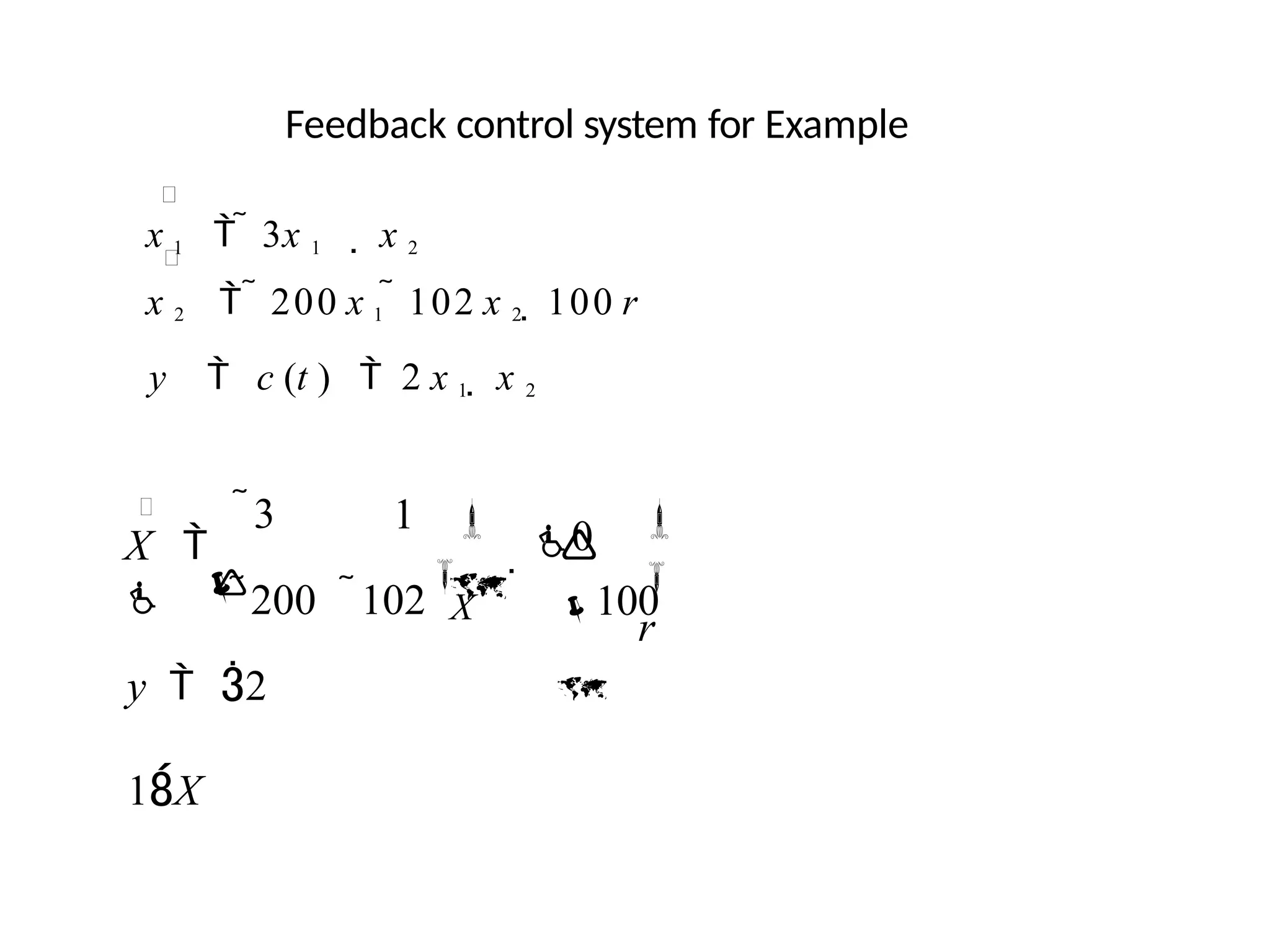
![State-space forms for
C(s)/R(s) =(s+ 3)/[(s+ 4)(s+ 6)].
Note: y = c(t)](https://image.slidesharecdn.com/pptcse1-250114082557-b9789d18/75/ppt-on-Control-system-engineering-1-pptx-113-2048.jpg)
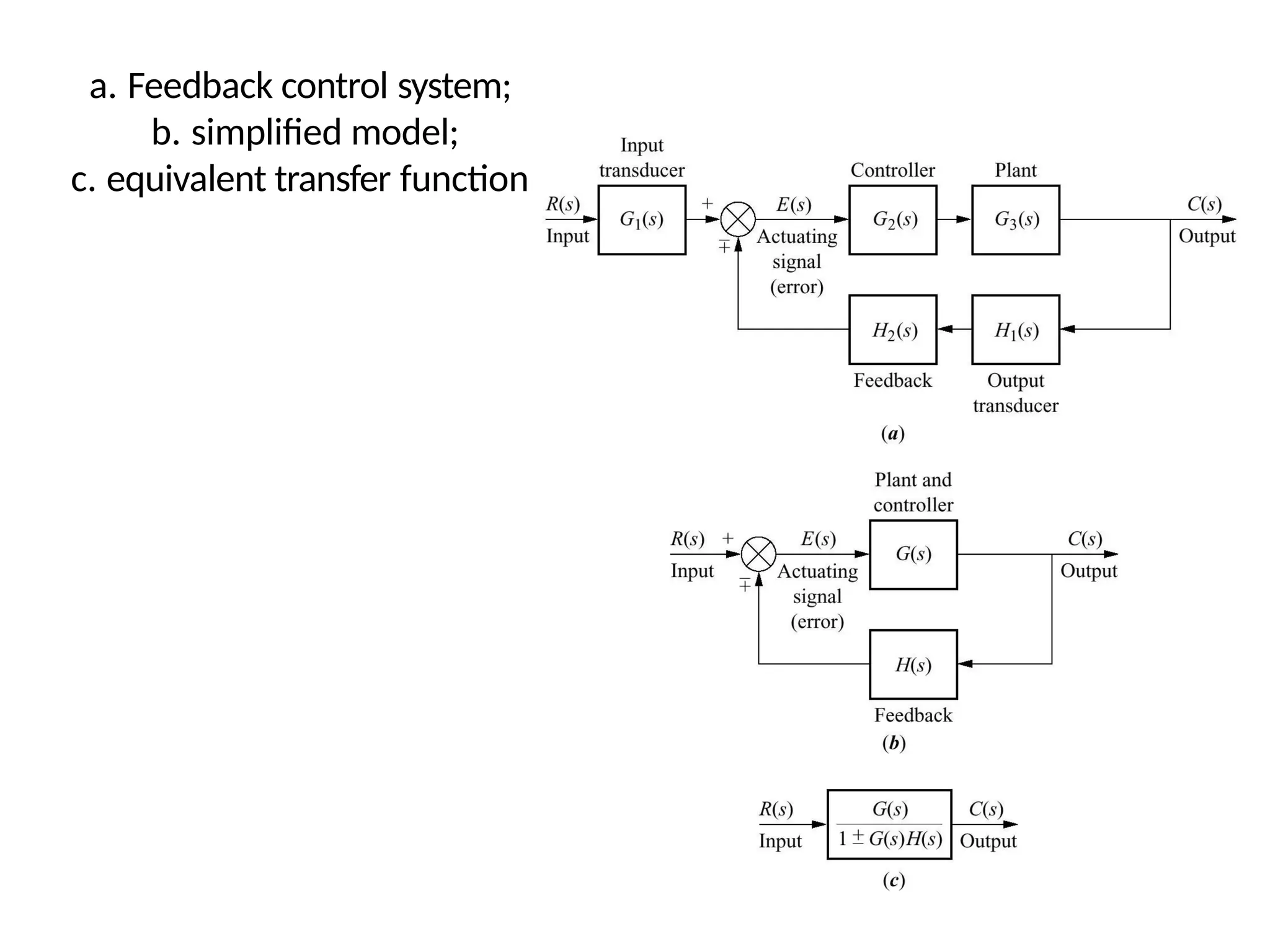
![Open-And Closed-Loop Control Systems
H ( s ) 1
Y ( s )
G ( s )
1 G ( s )
R ( s
)
E ( s )
1 G ( s )
1
R ( s )
T h u s , t o r e d u c e t h e e r r o r, t h e m a g n i t u d e
o f
1 G ( s ) 1
H ( s ) 1
Y ( s )
G ( s )
1 H ( s ) G ( s )
R ( s
)
E ( s )
1
1
H [ ( s ) G ( s ) ]
R ( s
)
T h u s , t o r e d u c e t h e e r r o r, t h e m a g n i t u d e
o f
1 G ( s ) H ( s ) 1
Error Signal](https://image.slidesharecdn.com/pptcse1-250114082557-b9789d18/75/ppt-on-Control-system-engineering-1-pptx-117-2048.jpg)
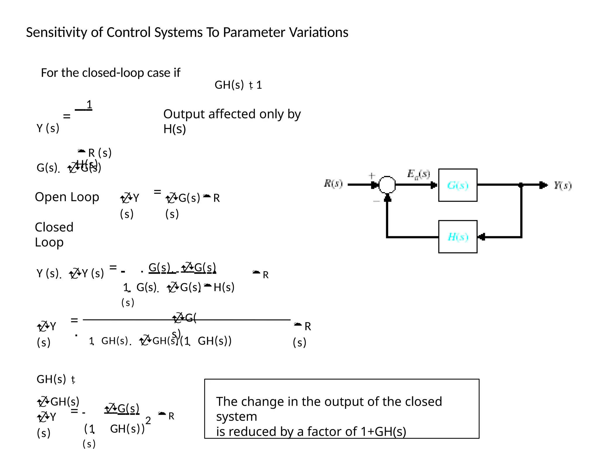
![Sensitivity of Control Systems To Parameter Variations
T ( s )
Y ( s )
R (
s )
S
T
( s )
T ( s )
G ( s )
G ( s )
S
d
T d
T
T
d
G
d
G
G
d
T
d T
G
G
d
G
d
T
T ( s )
1 1
H [ (
s ) G ( s ) ]
S G
d
T
G
d
G
d
T
d
T
G
d
G
d
T
( 1 GH )
2
G
( 1 GH )
T d T
G d T
G 1
G
S G
T 1
( 1
GH )
T GH
( 1
Sensitivity of the closed-loop to G variations
reduced
Sensitivity of the closed-loop to H variations
When GH is large sensitivity approaches 1
Changes in H directly affects the output
response
S H](https://image.slidesharecdn.com/pptcse1-250114082557-b9789d18/75/ppt-on-Control-system-engineering-1-pptx-119-2048.jpg)


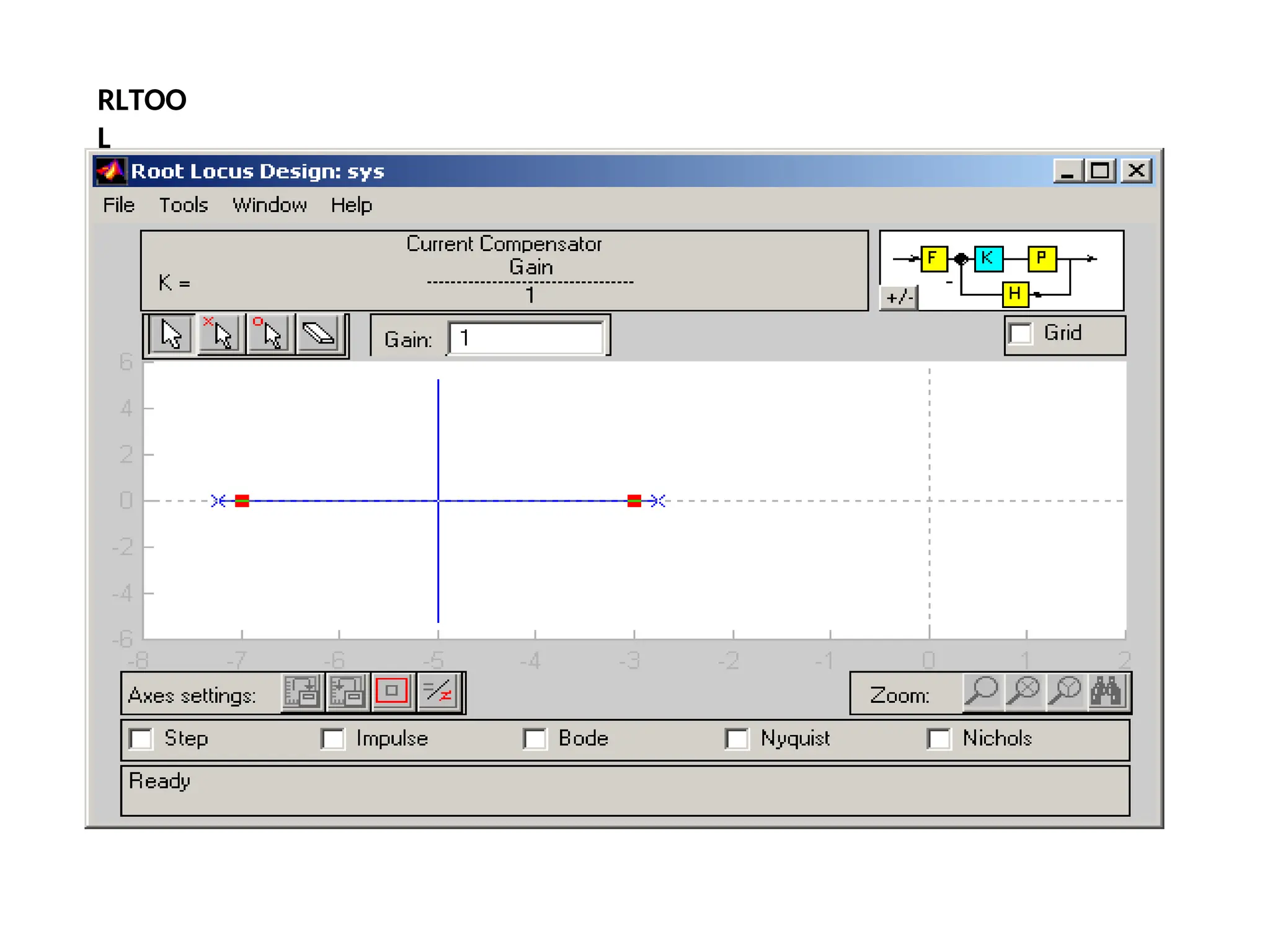
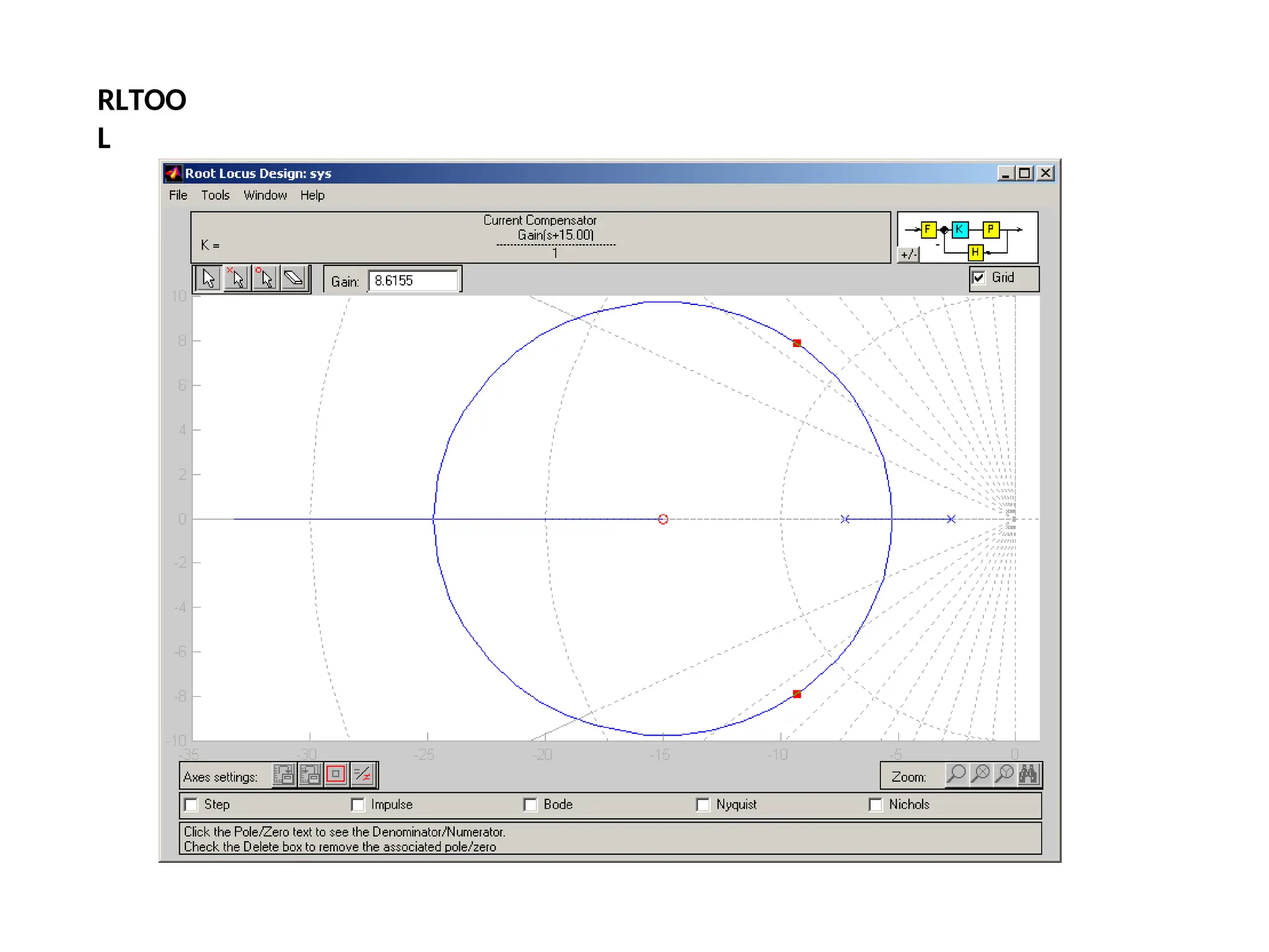
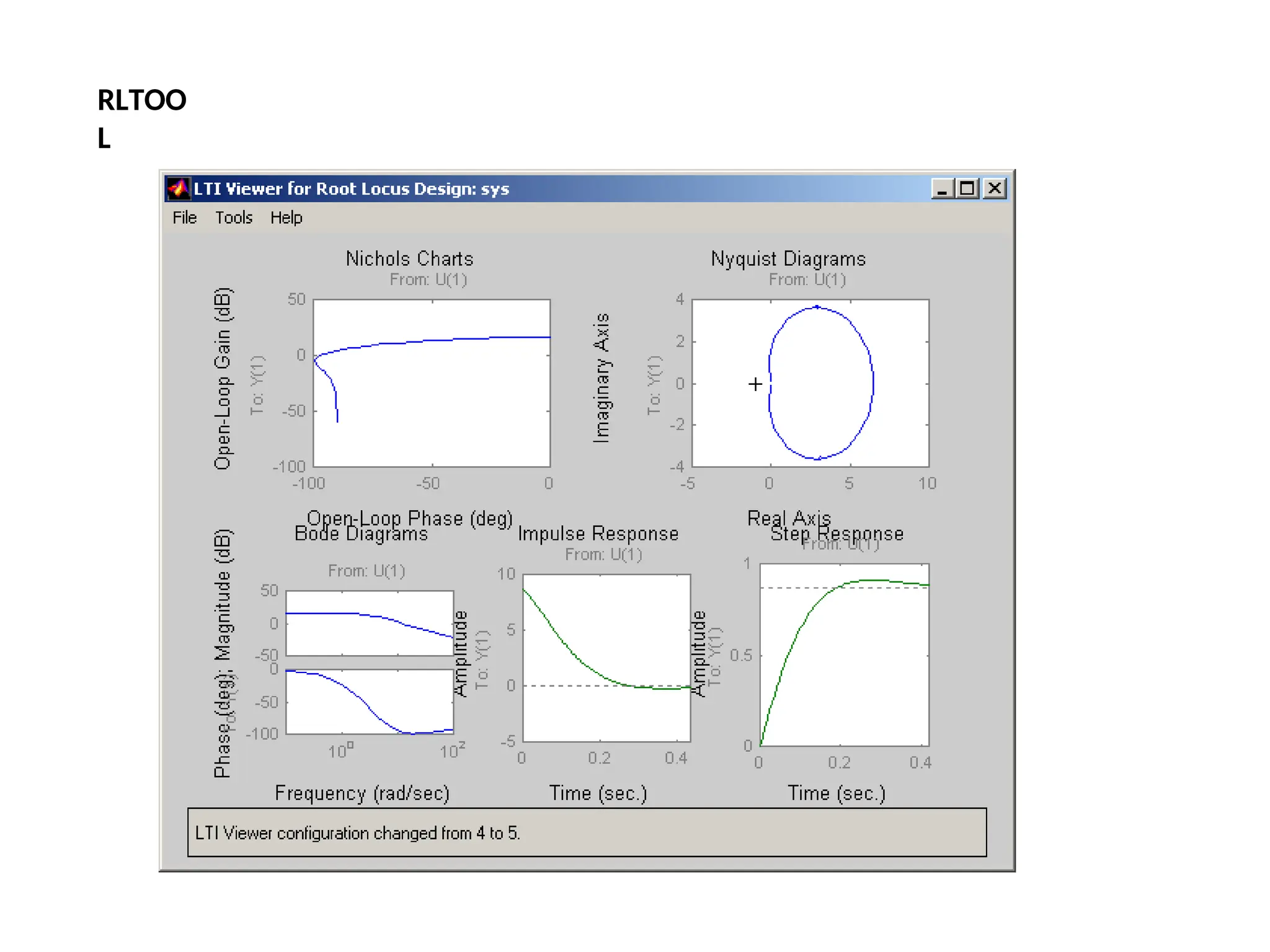
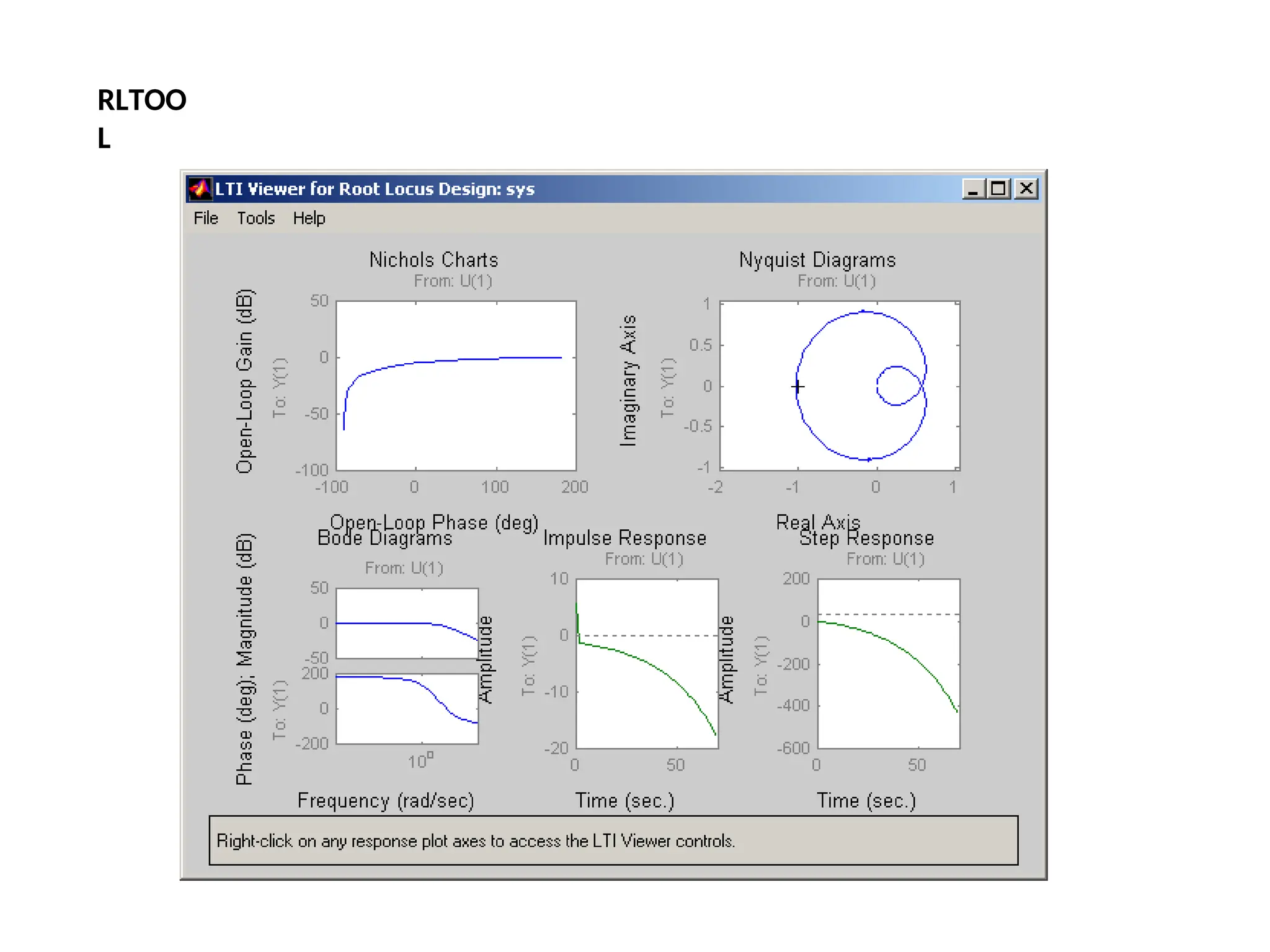
![MATLAB Example - Plotting the root locus of a transfer function
Consider an open loop system which has a transfer function of
G(s) = (s+7)/s(s+5)(s+15)(s+20)
How do we design a feedback controller for the system by
using the root locus method?
Enter the transfer function, and the command to plot the root
locus:
num=[1 7];
den=conv(conv([1 0],[1 5]),conv([1 15],
[1 20]));
rlocus(num,den)
axis([-22 3 -15 15])
Example](https://image.slidesharecdn.com/pptcse1-250114082557-b9789d18/75/ppt-on-Control-system-engineering-1-pptx-174-2048.jpg)

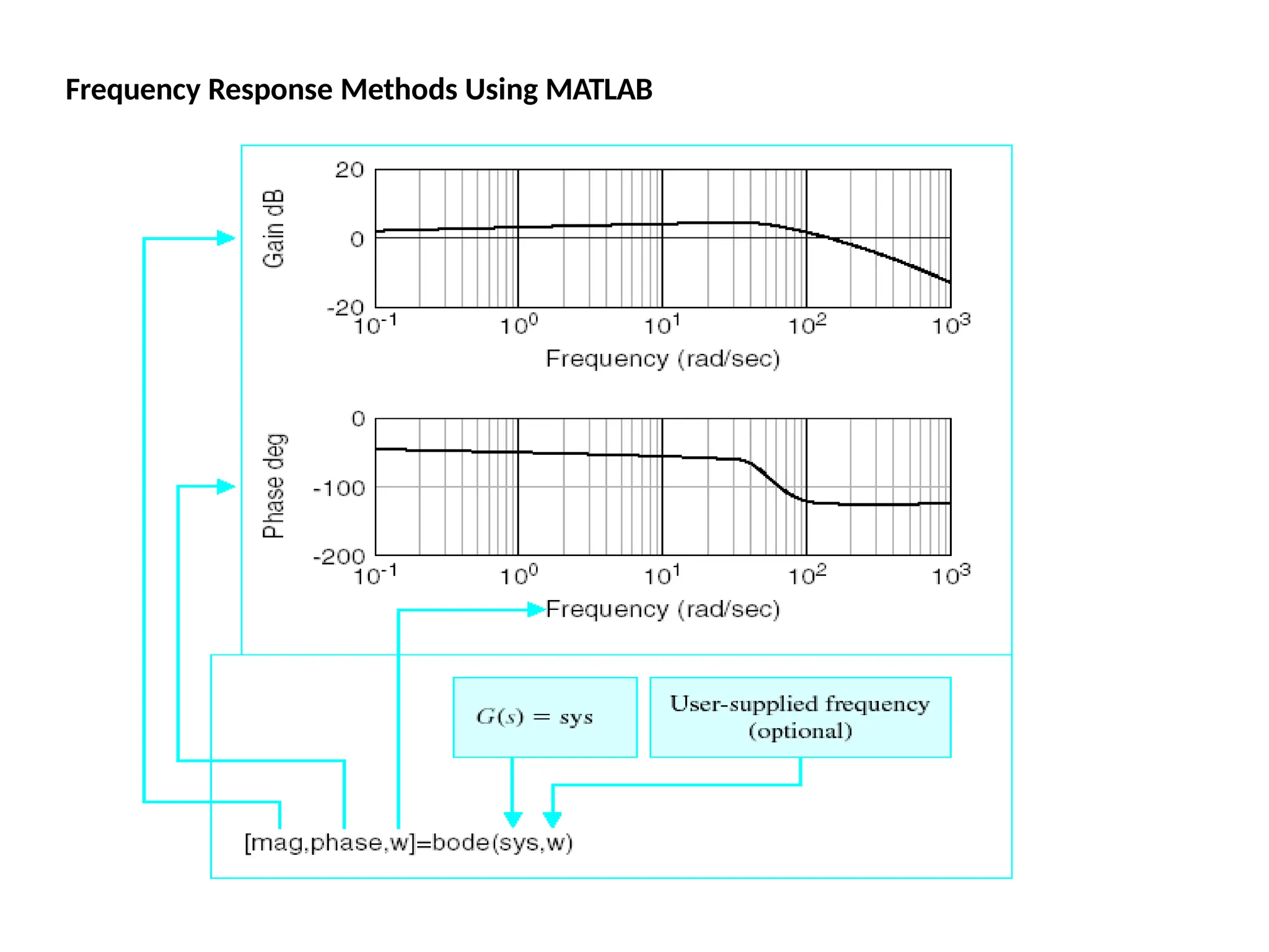
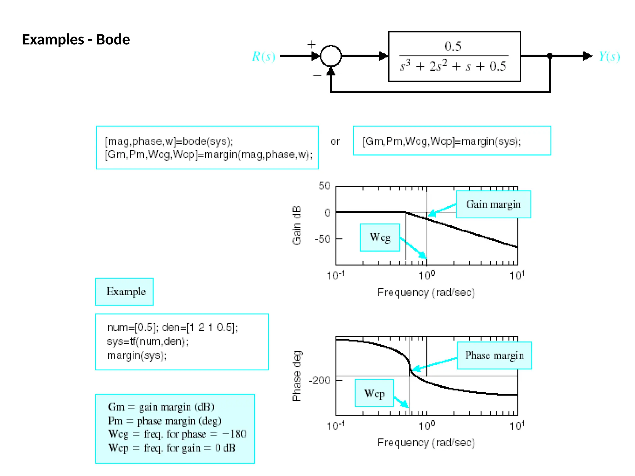
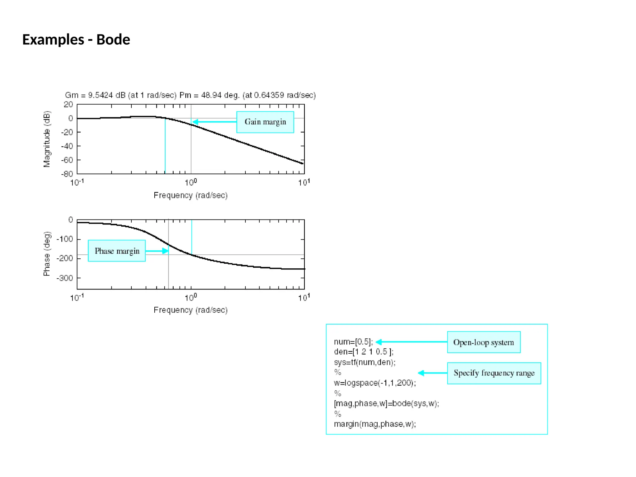
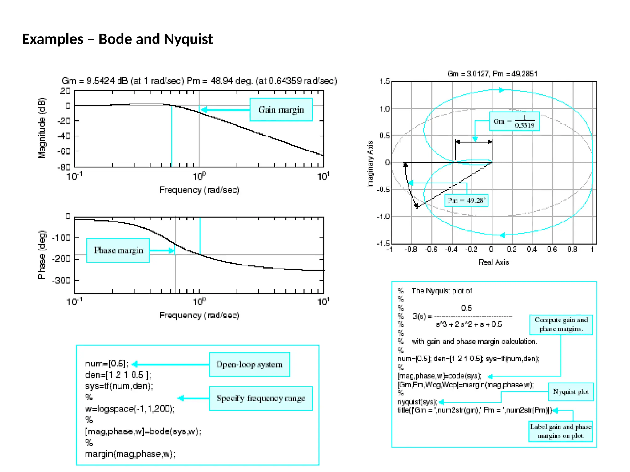
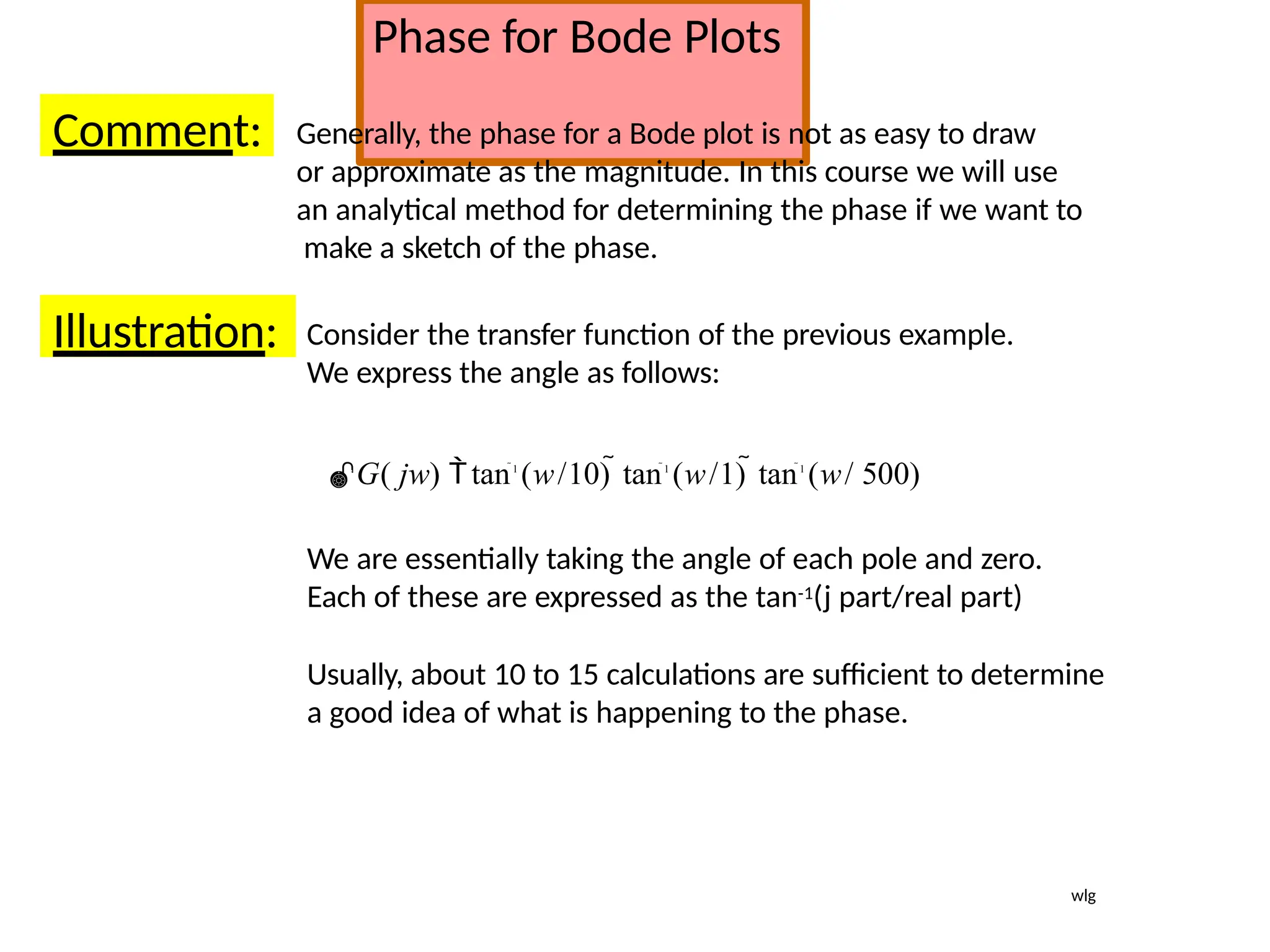
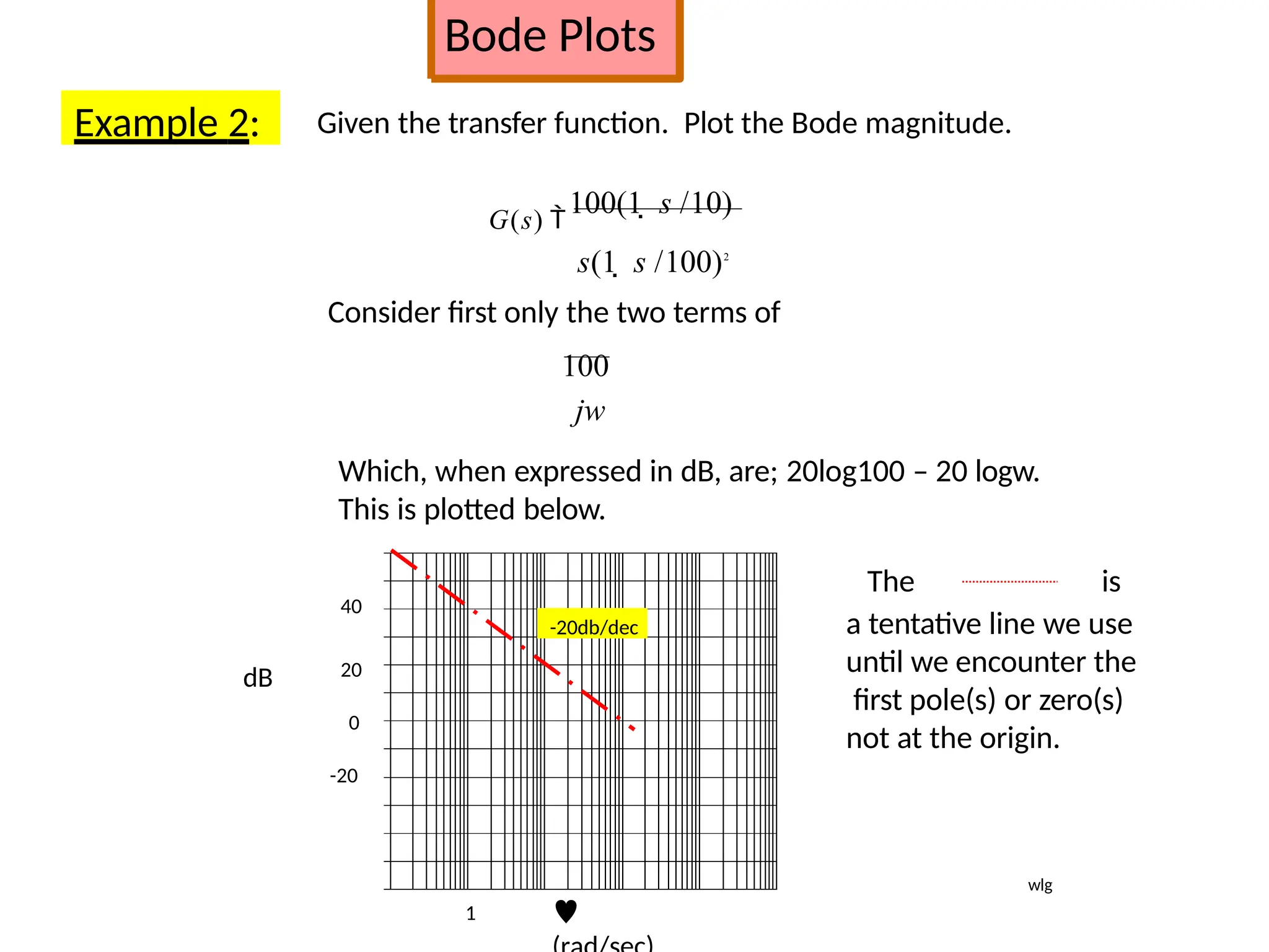
![Bode Plots
Bode plot is the representation of the magnitude and phase of G(j*w) (where
the frequency vector w contains only positive frequencies).
To see the Bode plot of a transfer function, you can use the MATLAB
bode
command.
For example,
bode(50,[1 9 30
40])
displays the Bode plots for the
transfer function:
50 / (s^3 + 9 s^2 + 30 s + 40)](https://image.slidesharecdn.com/pptcse1-250114082557-b9789d18/75/ppt-on-Control-system-engineering-1-pptx-216-2048.jpg)
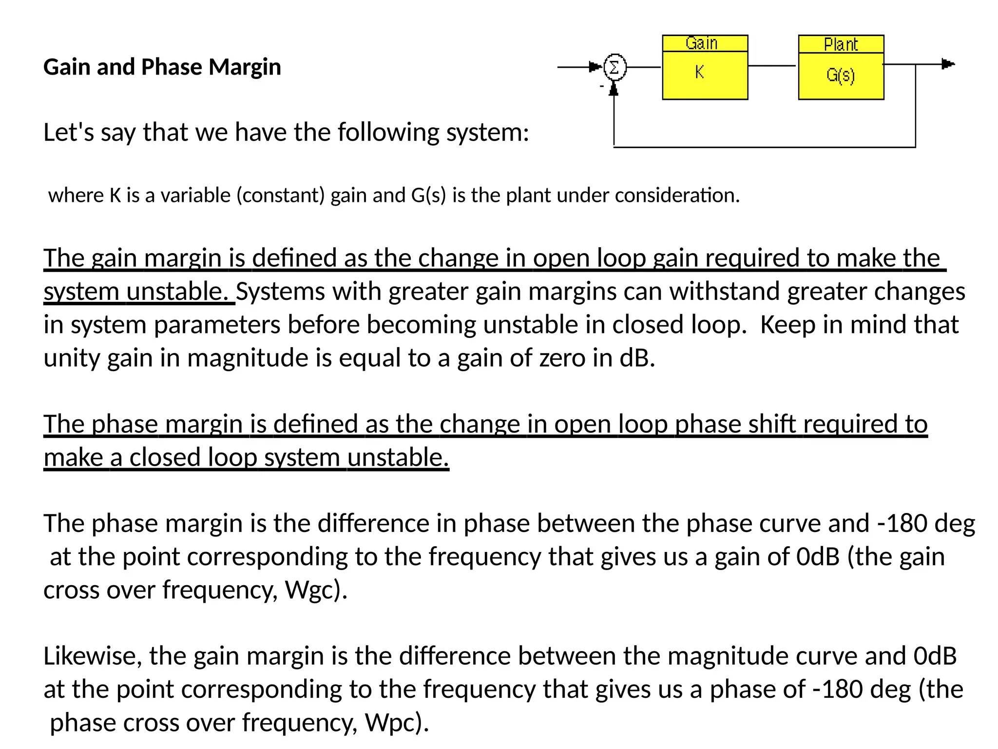
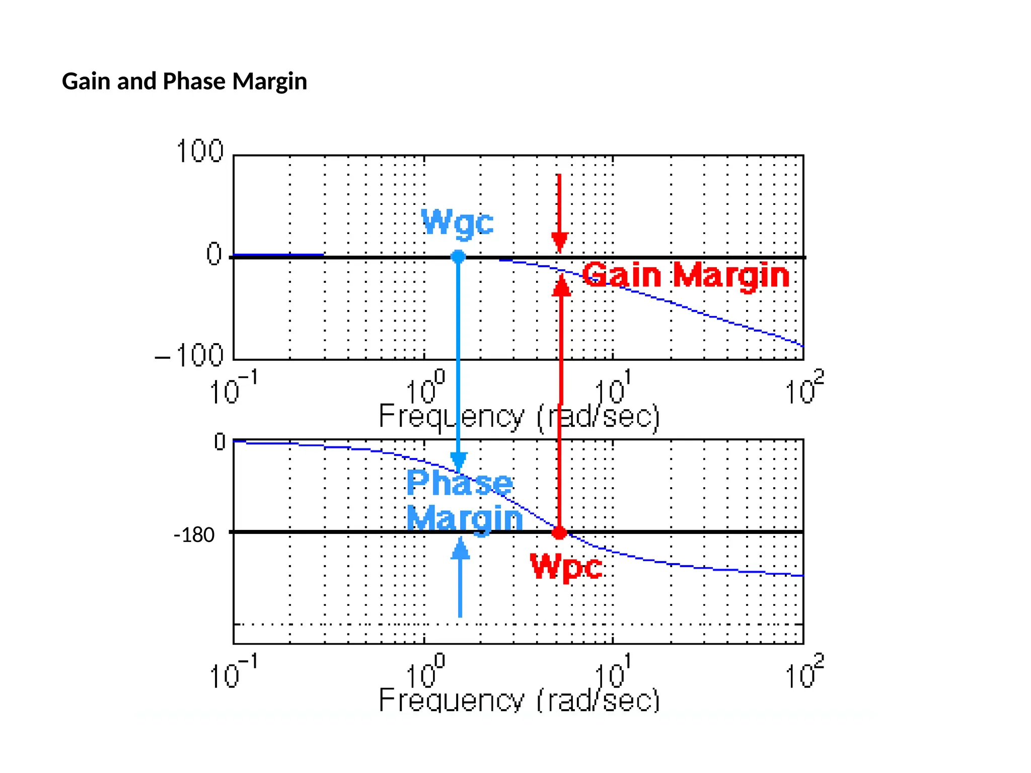
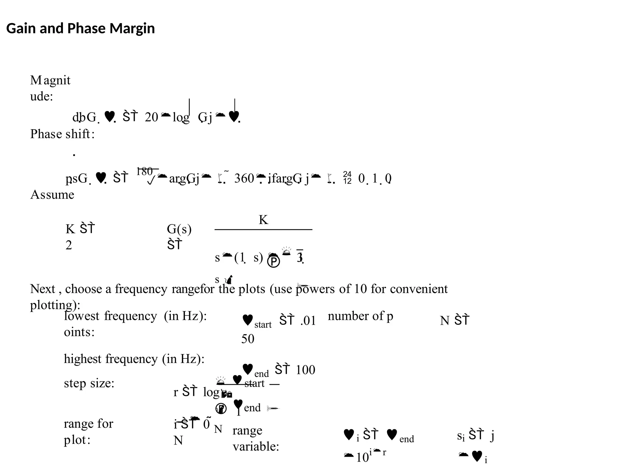
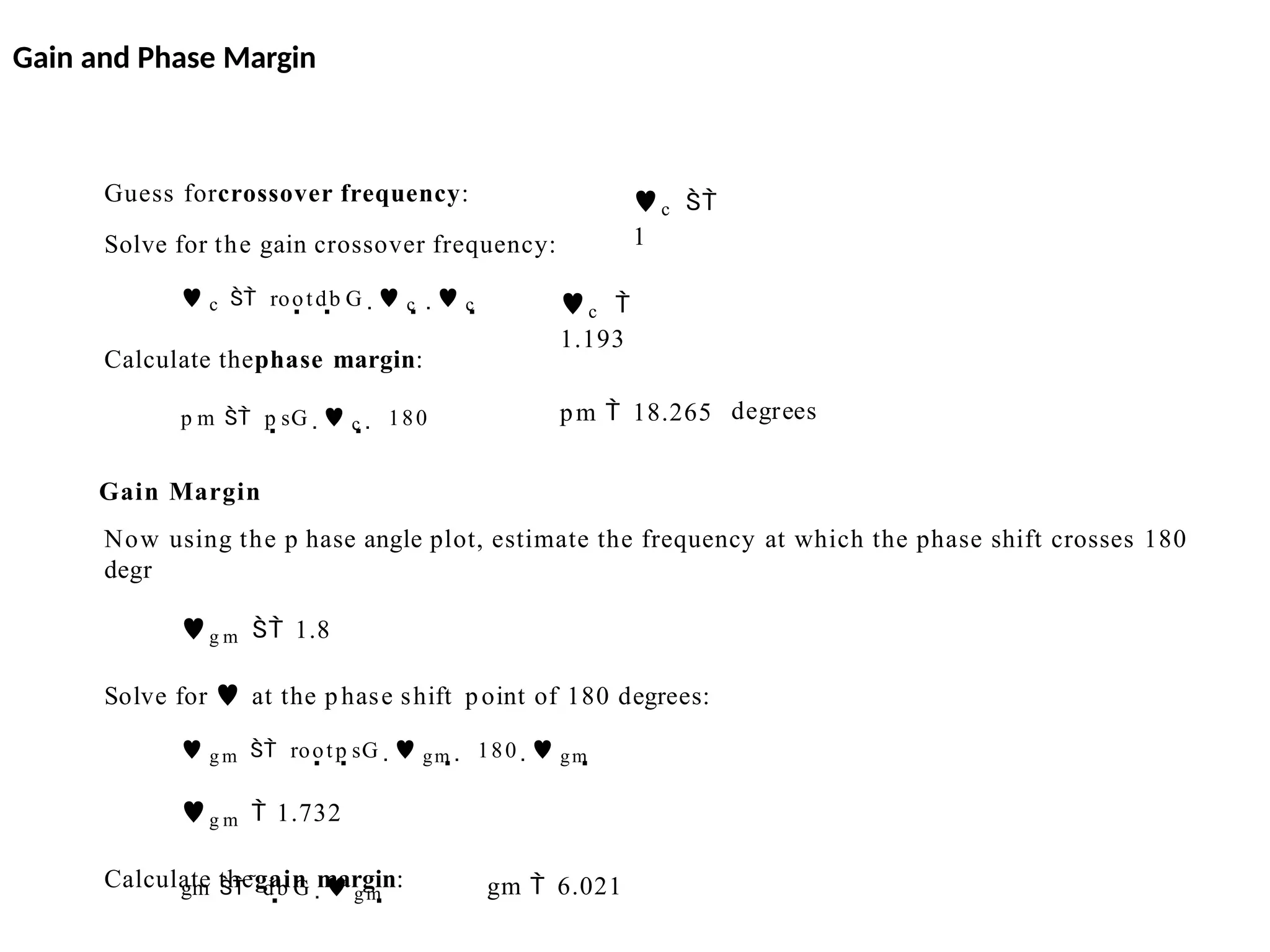
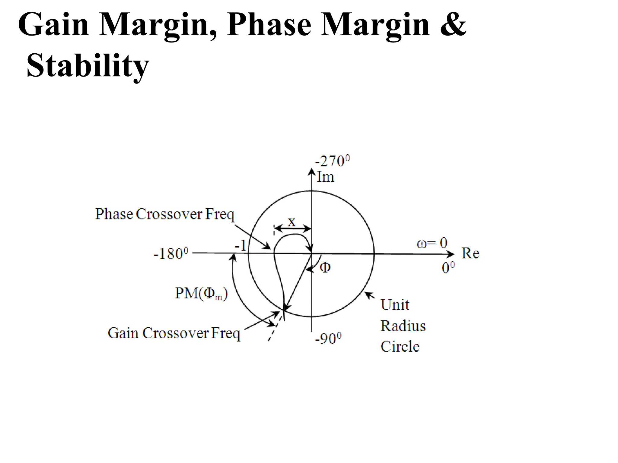
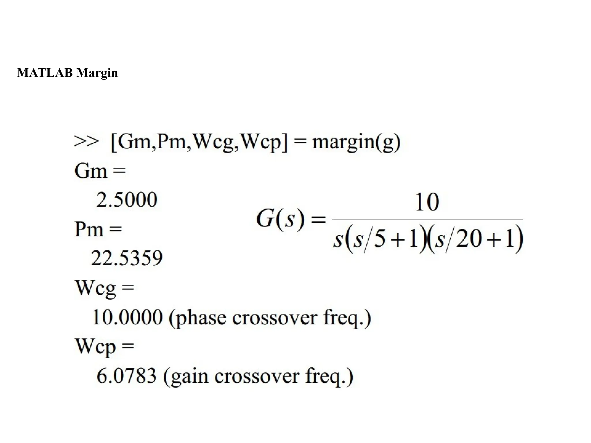
![We can find the gain and phase margins for a system directly, by using MATLAB.
Just enter the margin command.
e
This command returns the gain
and phase margins, the gain and
phase cross over frequencies, and
a graphical representation of
thes on the Bode plot.
margin(50,[1 9 30 40])
Gain and Phase Margin](https://image.slidesharecdn.com/pptcse1-250114082557-b9789d18/75/ppt-on-Control-system-engineering-1-pptx-219-2048.jpg)
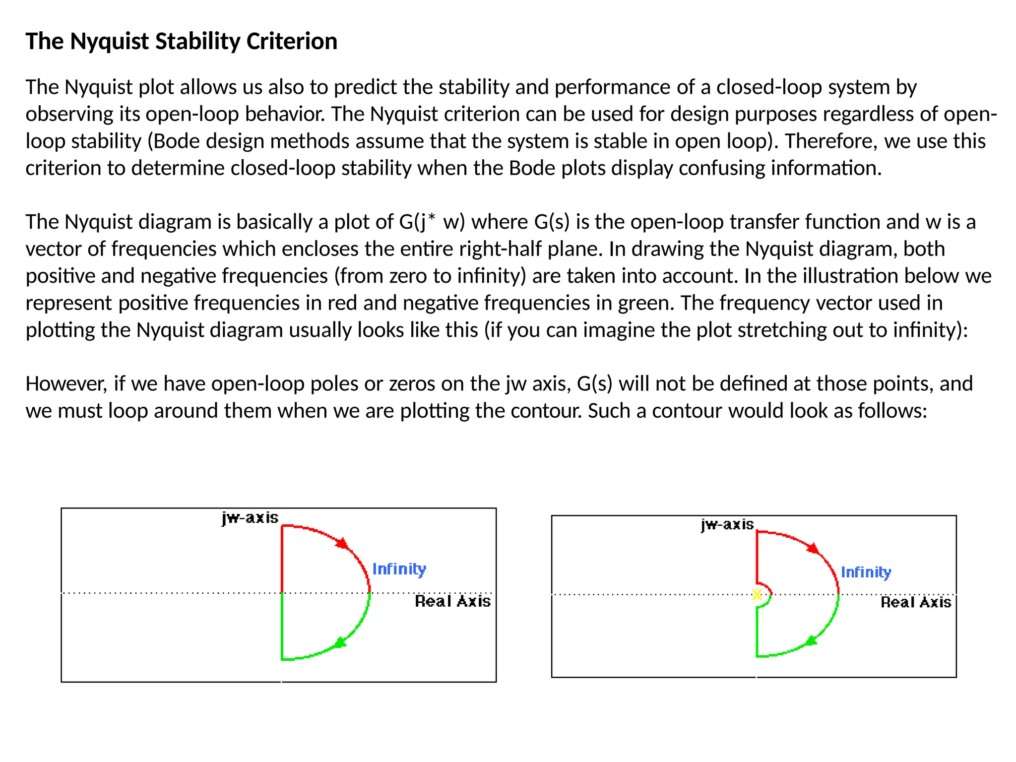
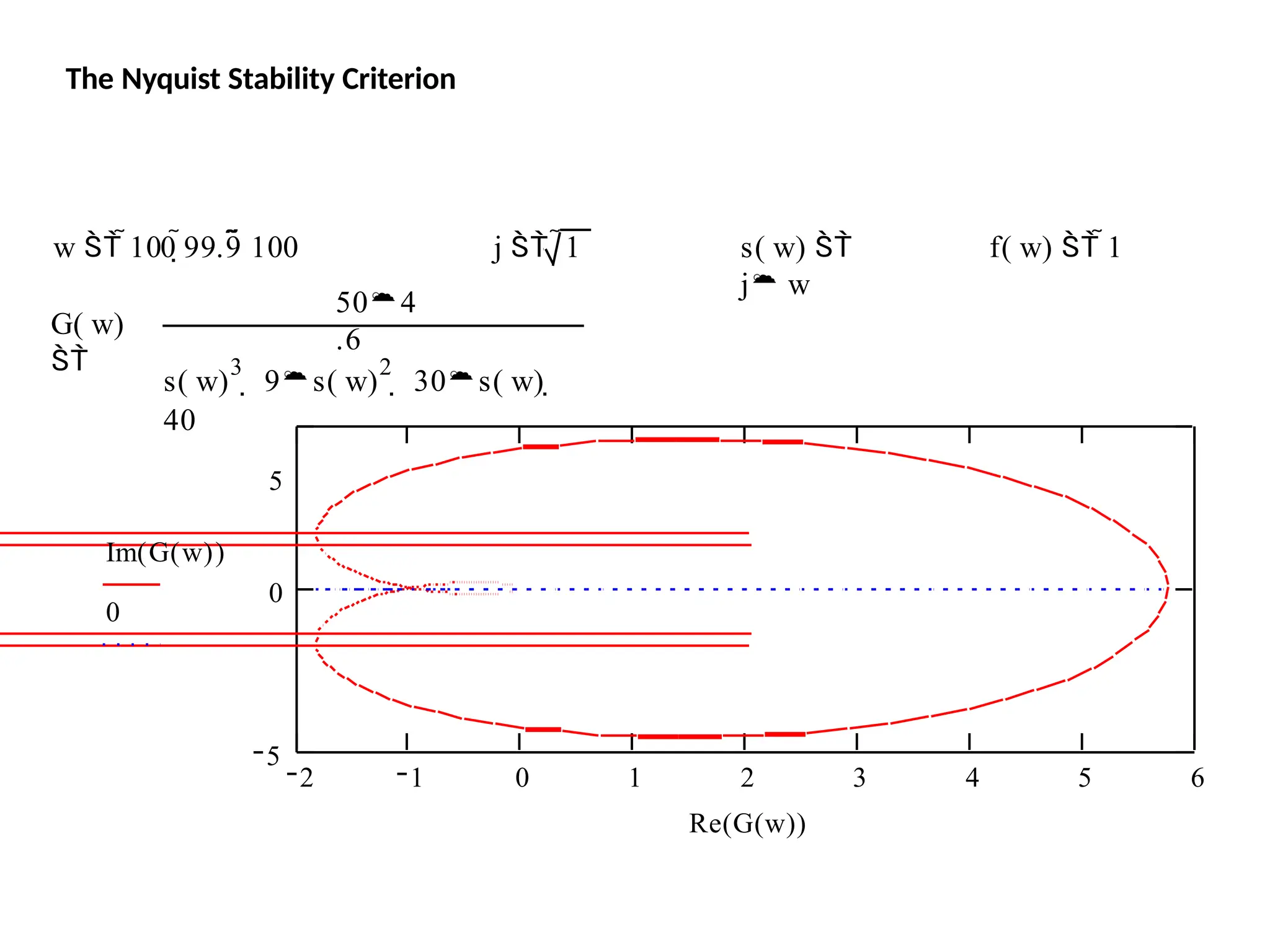
![and that the Nyquist diagram can be viewed by typing:
nyquist (50, [1 9 30 40 ])
The Nyquist Stability Criterion](https://image.slidesharecdn.com/pptcse1-250114082557-b9789d18/75/ppt-on-Control-system-engineering-1-pptx-225-2048.jpg)
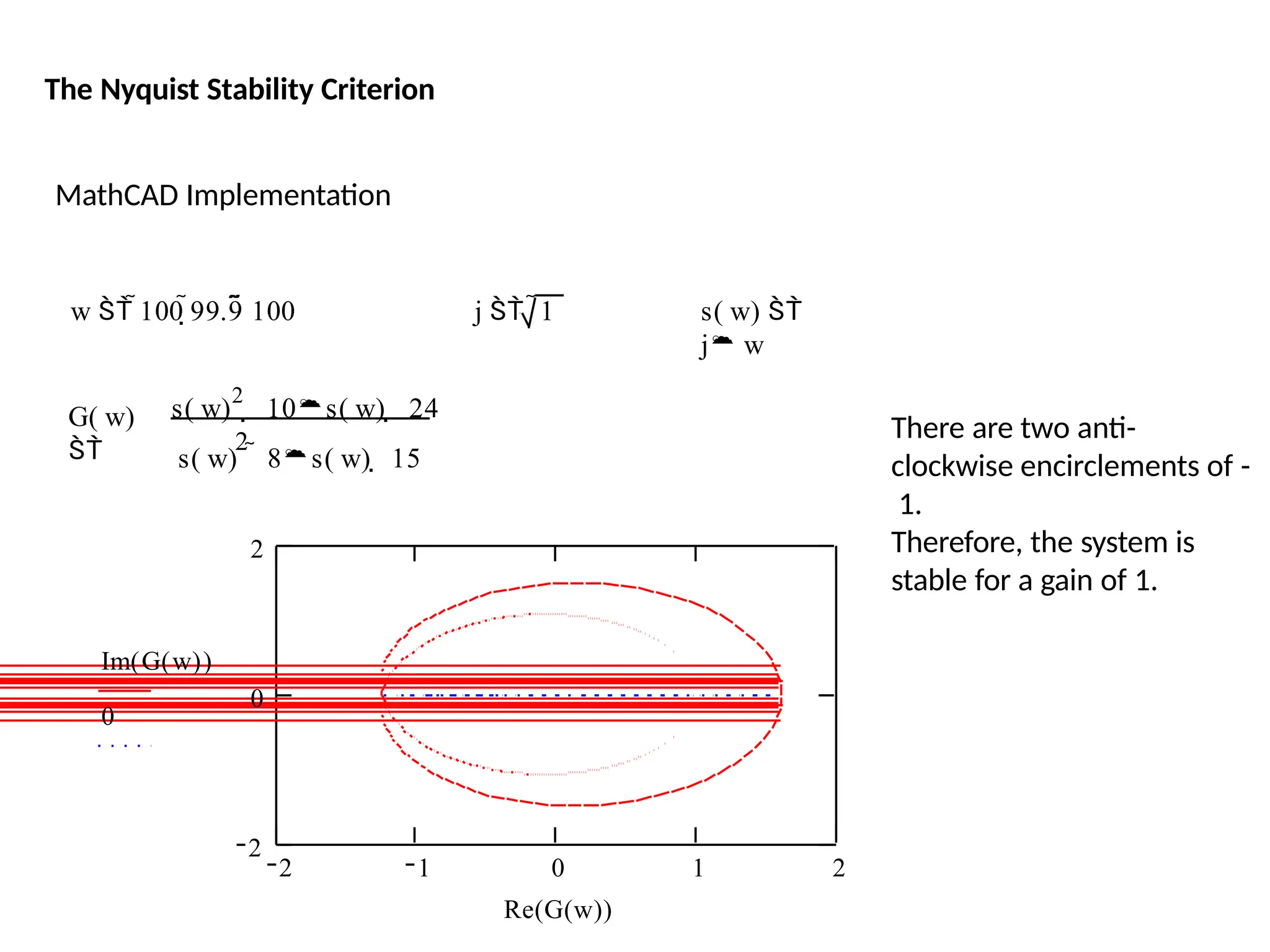
![This system has a gain K which can be varied in order to modify the response of the closed-loop
system. However, we will see that we can only vary this gain within certain limits, since we have to
make sure that our closed-loop system will be stable. This is what we will be looking for: the range
of gains that will make this system stable in the closed loop.
The first thing we need to do is find the number of positive real poles in our open-loop transfer
function:
roots([1 -8 15])
ans =
5
3
The poles of the open-loop transfer function are both positive. Therefore, we need two anti-
clockwise (N = -2) encirclements of the Nyquist diagram in order to have a stable closed-loop
system (Z = P + N). If the number of encirclements is less than two or the encirclements are not
anti-clockwise, our system will be unstable.
Let's look at our Nyquist diagram for a gain of 1:
nyquist([ 1 10 24], [ 1 -8 15])
There are two anti-clockwise encirclements of -1.
Therefore, the system is stable for a gain of 1.
The Nyquist Stability Criterion](https://image.slidesharecdn.com/pptcse1-250114082557-b9789d18/75/ppt-on-Control-system-engineering-1-pptx-230-2048.jpg)
![num=1;
den=[1 10
20];
step
(num,den)
Open-Loop Control - Example
G(s
)
1
s
2
10s 20](https://image.slidesharecdn.com/pptcse1-250114082557-b9789d18/75/ppt-on-Control-system-engineering-1-pptx-256-2048.jpg)
![Proportional Control - Example
The proportional controller (Kp) reduces the rise time, increases the overshoot, and
reduces the steady-state error.
MATLAB Example
Kp=300;
num=[Kp];
den=[1 10 20+Kp];
t=0:0.01:2;
step(num,den,t)
Amplitud
e
Step Response
From: U(1)
0 0.2 0.4 0.6 0.8 1
Time (sec.)
1.2 1.4 1.6 1.8 2
0
0.2
0.4
0.6
0.8
1
1.2
1.4
To:
Y(1)
T(s)
Kp
s
2
10s (20 Kp)
Amplitude
0 0.2 0.4 0.6 0.8 1
1.2
Time (sec.)
1.4 1.6 1.8 2
0
0.1
0.2
0.3
0.4
0.5
0.6
0.7
0.8
0.9
1
Step
Response
From: U(1)
To:
Y(1)
K=300 K=100](https://image.slidesharecdn.com/pptcse1-250114082557-b9789d18/75/ppt-on-Control-system-engineering-1-pptx-257-2048.jpg)
![Amplitud
e
Step Response
From: U(1)
0 0.2 0.4 0.6 0.8 1
Time (sec.)
1.2 1.4 1.6 1.8 2
0
0.2
0.4
0.6
0.8
1
1.2
1.4
To:
Y(1)
Kp=300;
Kd=10;
num=[Kd Kp];
den=[1 10+Kd 20+Kp];
t=0:0.01:2;
step(num,den,t)
Proportional - Derivative - Example
The derivative controller (Kd) reduces both the overshoot and the settling time.
MATLAB Example
T(s)
Kds
Kp
s
2
(10 Kd)s (20 Kp)
Amplitud
e
0 0.2 0.4
0.6
0.8 1
1.2
Time (sec.)
1.4 1.6 1.8 2
0
0.1
0.2
0.3
0.4
0.5
0.6
0.7
0.8
0.9
1
Step Response
From: U(1)
To:
Y(1)
Kd=10
Kd=20](https://image.slidesharecdn.com/pptcse1-250114082557-b9789d18/75/ppt-on-Control-system-engineering-1-pptx-258-2048.jpg)
![Proportional - Integral - Example
The integral controller (Ki) decreases the rise time, increases both the overshoot and the
settling time, and eliminates the steady-state error
MATLAB Example
Amplitud
e
Step Response
From: U(1)
0 0.2 0.4 0.6 0.8 1
Time (sec.)
1.2 1.4 1.6 1.8 2
0
0.4
0.6
0.8
1
1.2
1.4
To:
Y(1)
Kp=30;
Ki=70;
num=[Kp Ki];
den=[1 10 20+Kp Ki]; 0.2
t=0:0.01:2;
step(num,den,t)
T(s)
Kps
Ki
s3
10s2
(20 Kp)s Ki
Amplitud
e
0.2 0.4 0.6 0.8 1 1.2
Time (sec.)
1.4 1.6 1.8 2
0
0
0.2
0.4
0.6
0.8
1
1.2
1.4
Step Response
From: U(1)
To:
Y(1)
Ki=70
Ki=100](https://image.slidesharecdn.com/pptcse1-250114082557-b9789d18/75/ppt-on-Control-system-engineering-1-pptx-259-2048.jpg)
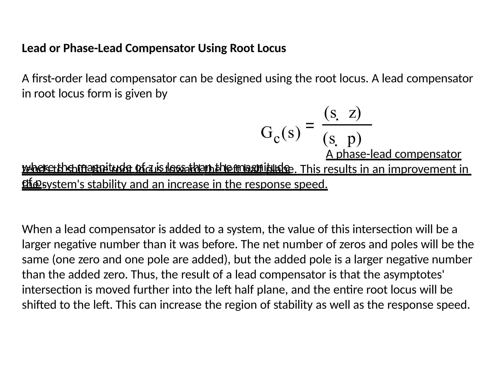
![In Matlab a phase lead compensator in root locus form is implemented by using the
transfer function in the form
numlead=kc*[1 z];
denlead=[1 p];
and using the conv() function to implement it with the numerator
and denominator of the plant
newnum=conv(num,numlead);
newden=conv(den,denlead);
Lead or Phase-Lead Compensator Using Root Locus](https://image.slidesharecdn.com/pptcse1-250114082557-b9789d18/75/ppt-on-Control-system-engineering-1-pptx-268-2048.jpg)
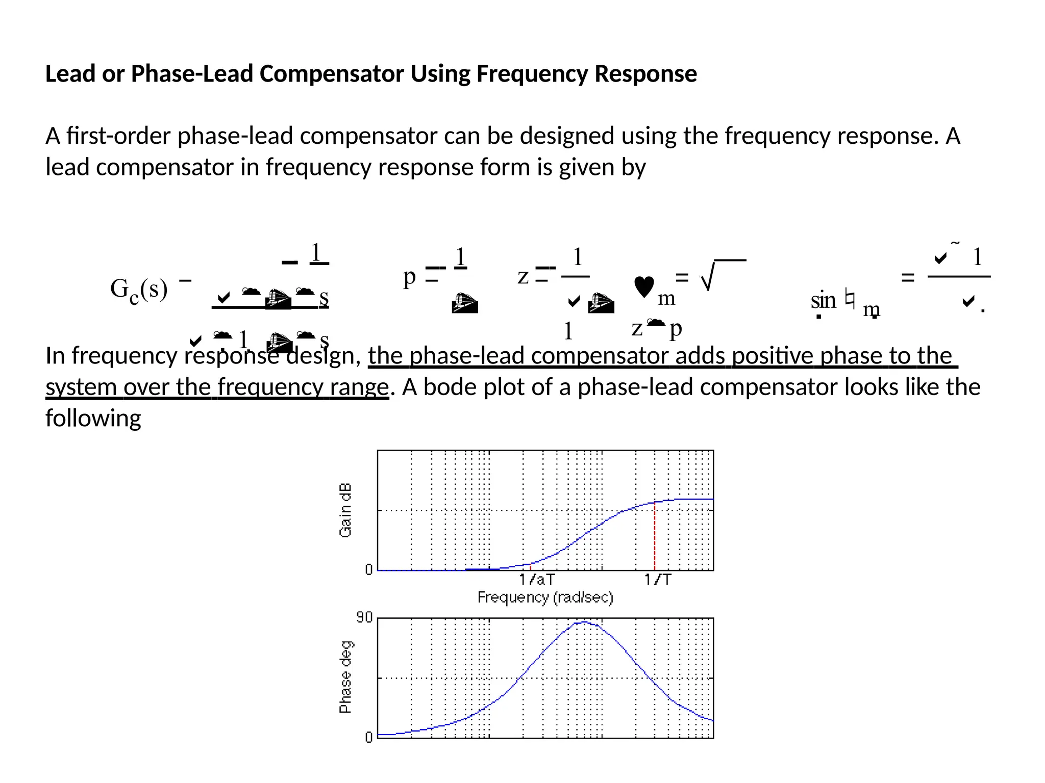
![In Matlab, a phase lead compensator in frequency response form is
implemented by using the transfer function in the form
numlead=[aT 1];
denlead=[T 1];
and using the conv() function to multiply it by the numerator
and denominator of the plant
newnum=conv(num,numlead);
newden=conv(den,denlead);
Lead or Phase-Lead Compensator Using Frequency Response](https://image.slidesharecdn.com/pptcse1-250114082557-b9789d18/75/ppt-on-Control-system-engineering-1-pptx-271-2048.jpg)
![It was previously stated that that lag controller should only minimally change the
transient response because of its negative effect. If the phase-lag compensator is
not supposed to change the transient response noticeably, what is it good for?
The answer is that a phase-lag compensator can improve the system's steady-state
response. It works in the following manner. At high frequencies, the lag controller
will have unity gain. At low frequencies, the gain will be z0/p0 which is greater
than 1. This factor z/p will multiply the position, velocity, or acceleration constant
(Kp, Kv, or Ka), and the steady-state error will thus decrease by the factor z0/p0.
In Matlab, a phase lead compensator in root locus form is implemented by using
the transfer function in the form
numlag=[1 z];
denlag=[1 p];
and using the conv() function to implement it with the numerator
and denominator of the plant
newnum=conv(num,numlag);
newden=conv(den,denlag);
Lag or Phase-Lag Compensator Using Root Locus](https://image.slidesharecdn.com/pptcse1-250114082557-b9789d18/75/ppt-on-Control-system-engineering-1-pptx-273-2048.jpg)
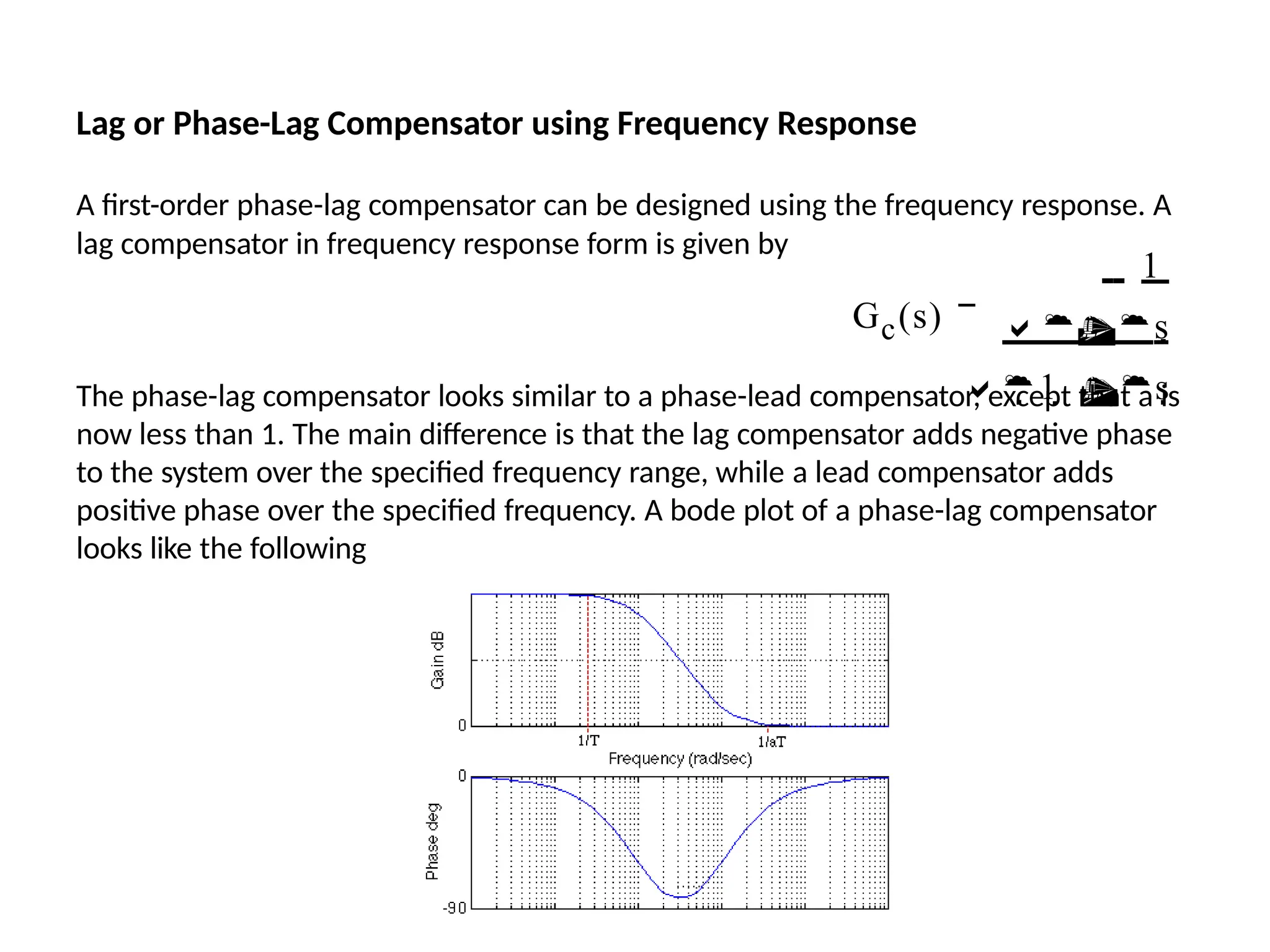
![In Matlab, a phase-lag compensator in frequency response form is
implemented by using the transfer function in the form
numlead=[a*T 1];
denlead=a*[T 1];
and using the conv() function to implement it with the numerator
and denominator of the plant
newnum=conv(num,numlead);
newden=conv(den,denlead);
Lag or Phase-Lag Compensator using Frequency Response](https://image.slidesharecdn.com/pptcse1-250114082557-b9789d18/75/ppt-on-Control-system-engineering-1-pptx-275-2048.jpg)
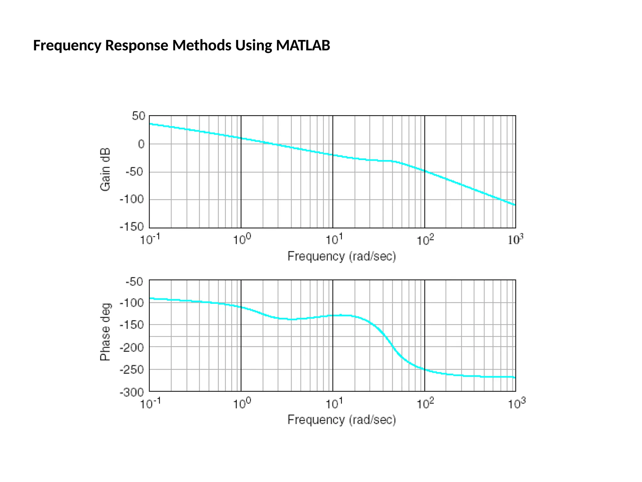
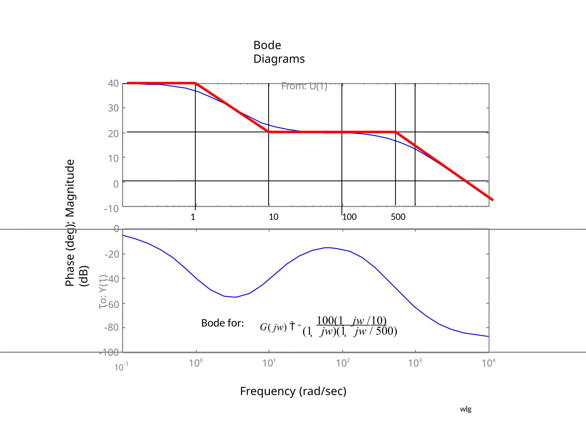
![Using Matlab For Frequency Response
Instruction: We can use Matlab to run the frequency response for
the previous example. We place the transfer function
in the form:
5000(s 10)
[5000s
50000]
(s 1)(s 500) [ s2
501s 500]
The Matlab Program
num = [5000 50000];
den = [1 501 500];
Bode (num,den)
In the following slide, the resulting magnitude and phase plots (exact)
are shown in light color (blue). The approximate plot for the magnitude
(Bode) is shown in heavy lines (red). We see the 3 dB errors at the
corner frequencies.
wlg](https://image.slidesharecdn.com/pptcse1-250114082557-b9789d18/75/ppt-on-Control-system-engineering-1-pptx-294-2048.jpg)
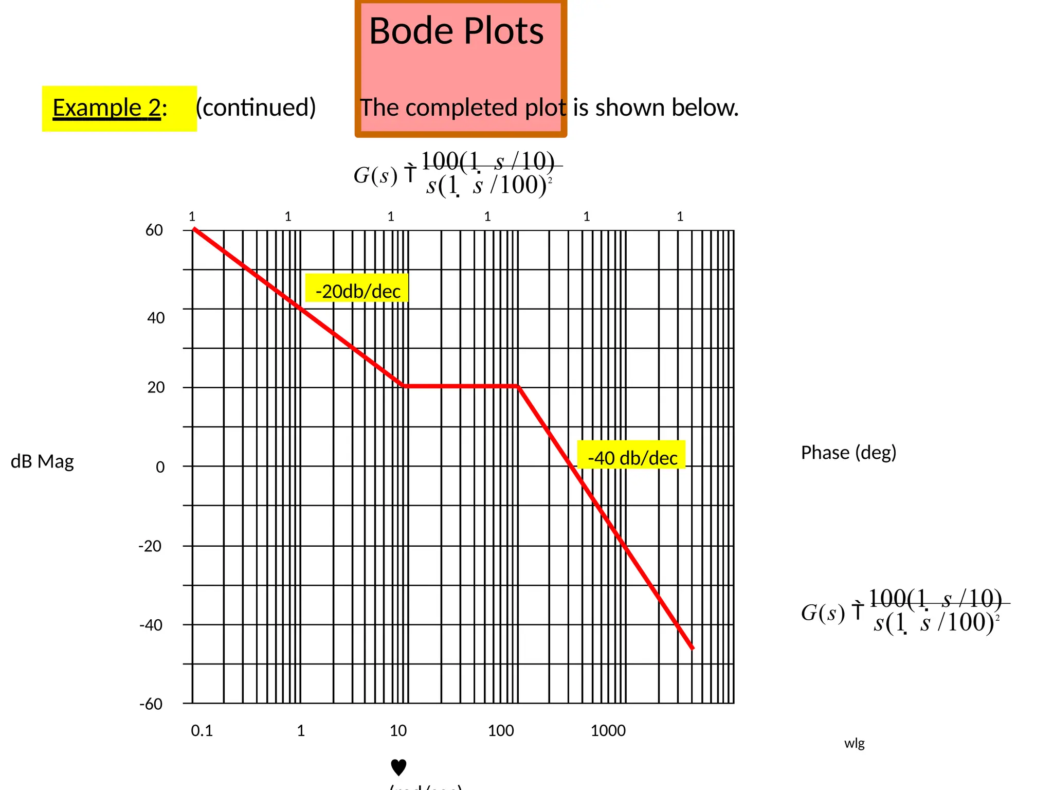
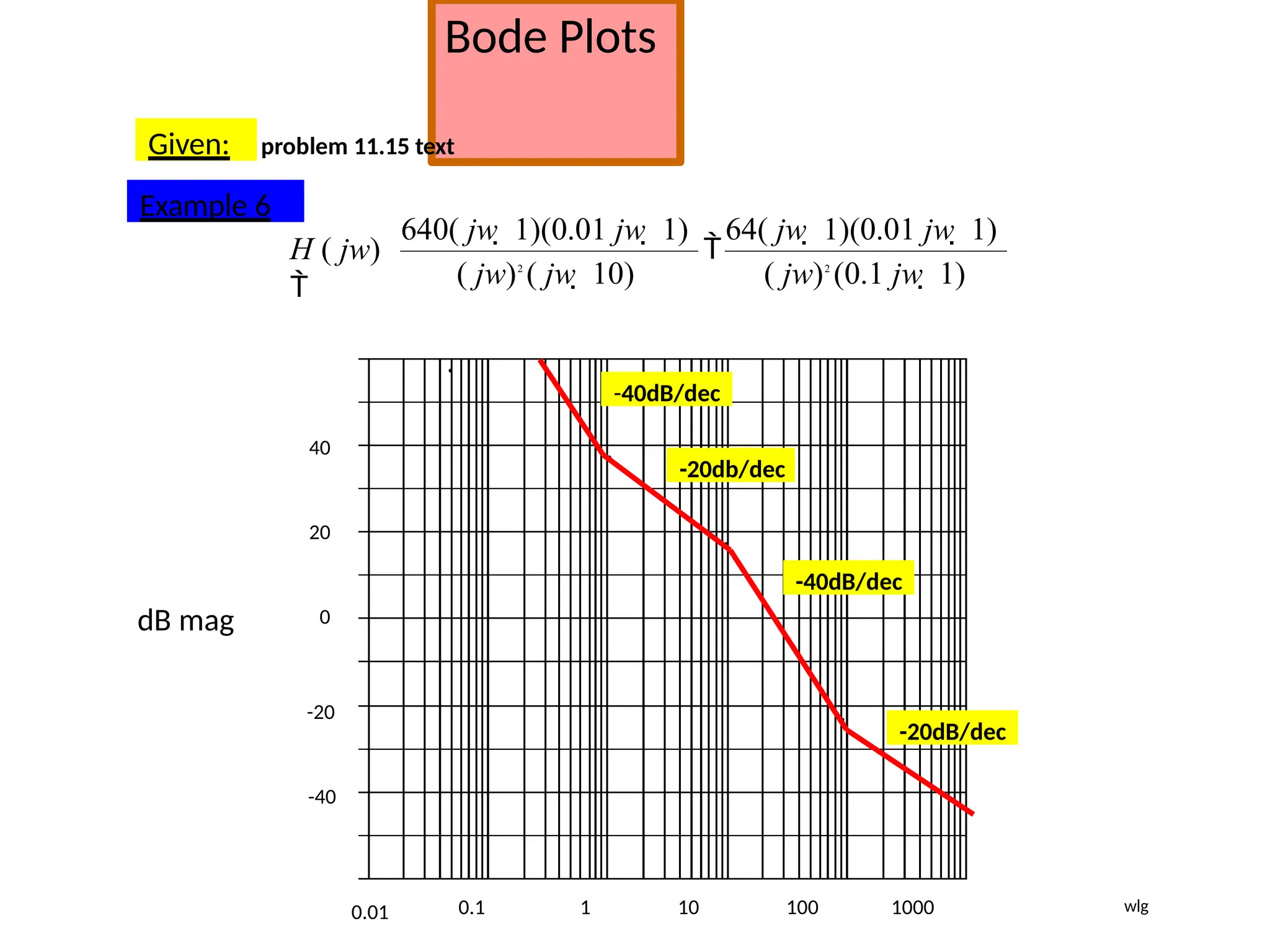
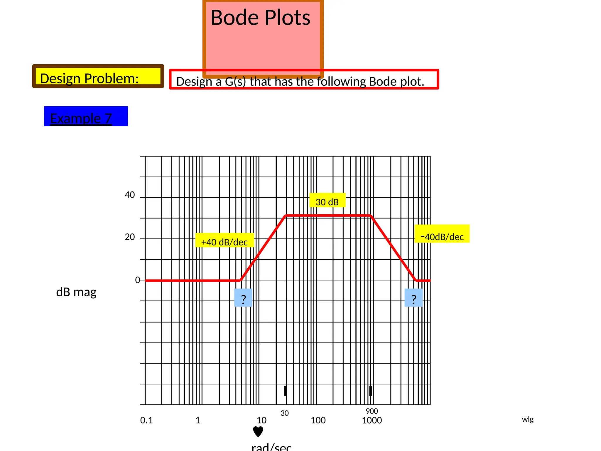
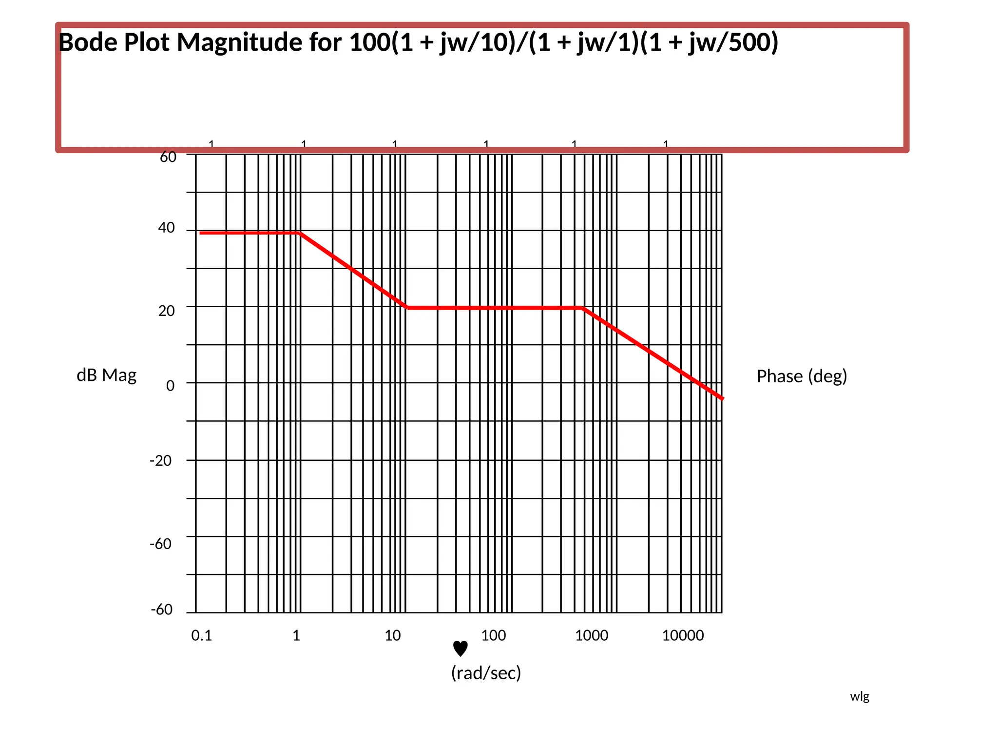
![Bode Plots
Procedure: The two break frequencies need to be found.
Recall:
#dec = log10[w2/w1]
Then we have:
(#dec)( 40dB/dec) = 30
dB
log10[w1/30] = 0.75 w1 = 5.33 rad/sec
Also:
log10[w2/900] (-40dB/dec) = - 30dB
This gives w2 = 5060 rad/sec
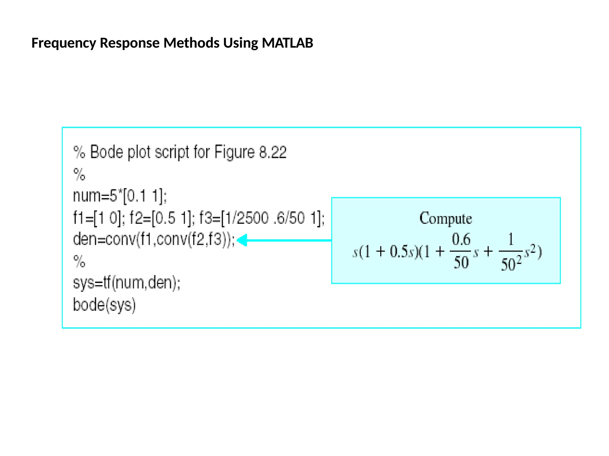
wlg](https://image.slidesharecdn.com/pptcse1-250114082557-b9789d18/75/ppt-on-Control-system-engineering-1-pptx-304-2048.jpg)
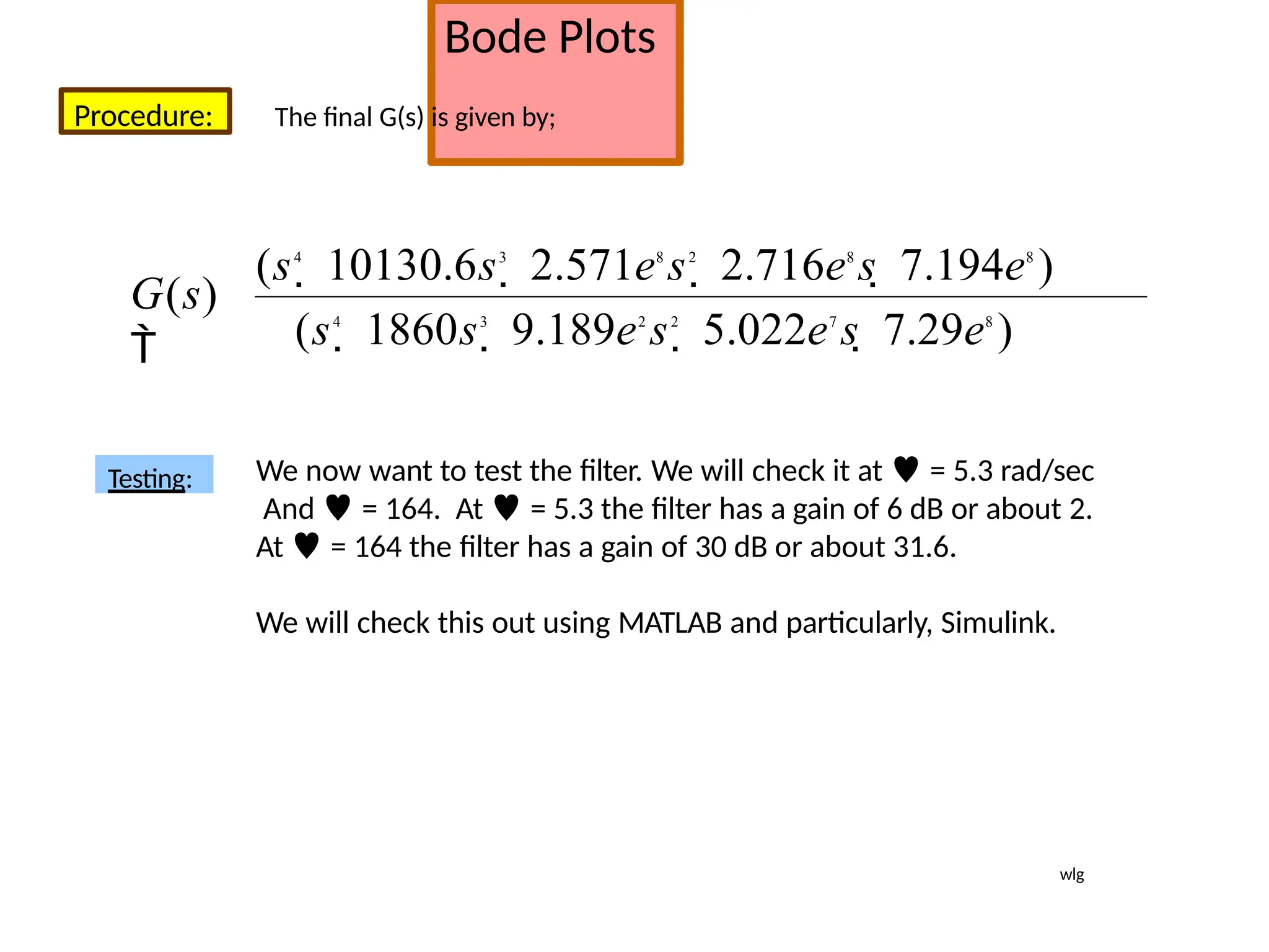
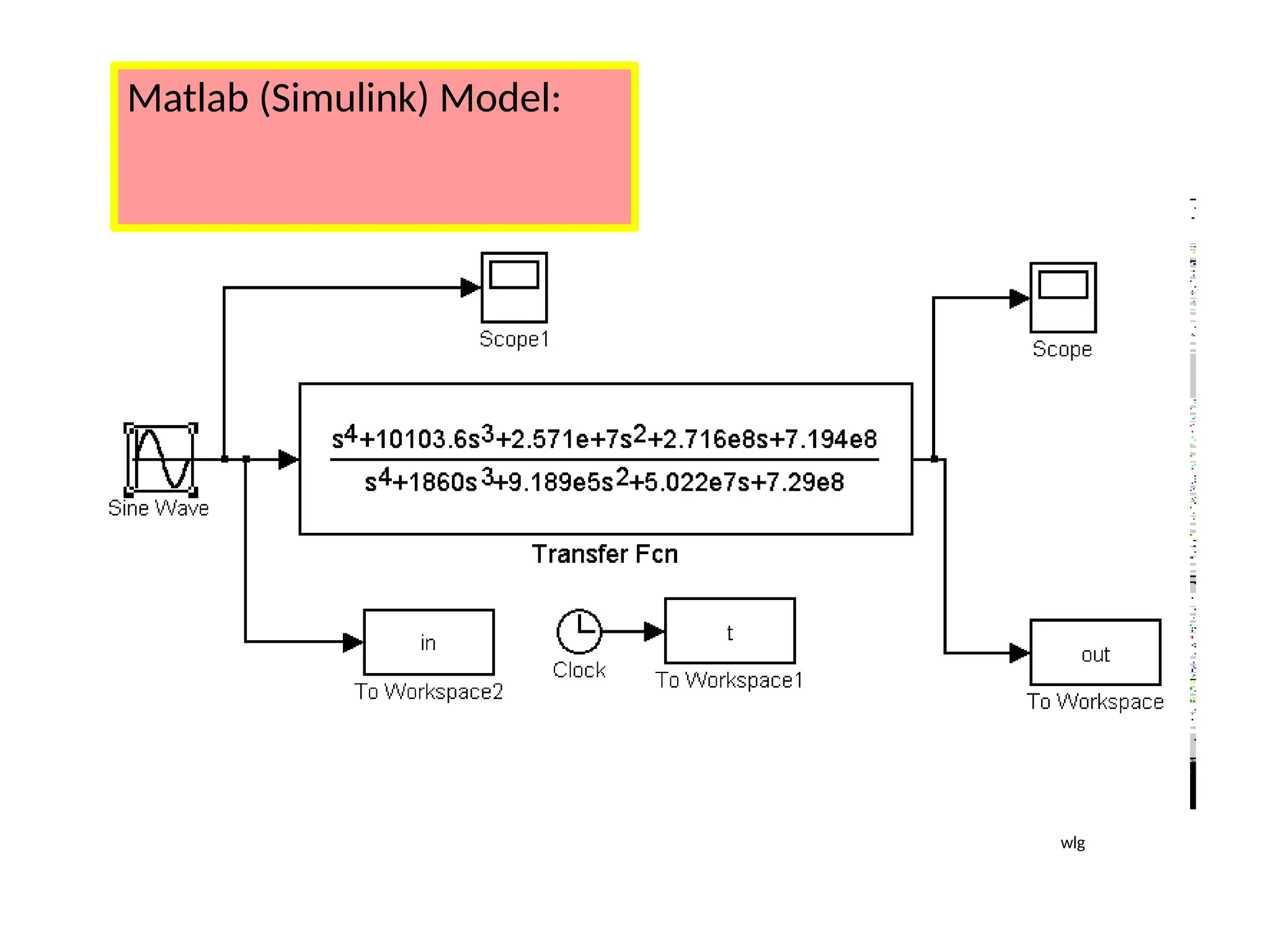
![Bode Plots
Procedure:
(1 s / 5.3)2
(1 s / 5060)2
G(s)
(1 s / 30)2
(1 s / 900)2
Clearing:
(s 5.3)2
(s 5060)2
G(s)
(s 30)2
(s 900)2
Use Matlab and conv:
N 2 (s2
10120s 2.56xe7
)
N2 = [1 10120 2.56e+7]
7.222e+8
s4
N1 (s2
10.6s 28.1)
N1 = [1 10.6 28.1]
N =
conv(N1,N2)
1 1.86e+3 2.58e+7 2.73e+8
s3 s2
s1
s0
wlg](https://image.slidesharecdn.com/pptcse1-250114082557-b9789d18/75/ppt-on-Control-system-engineering-1-pptx-305-2048.jpg)

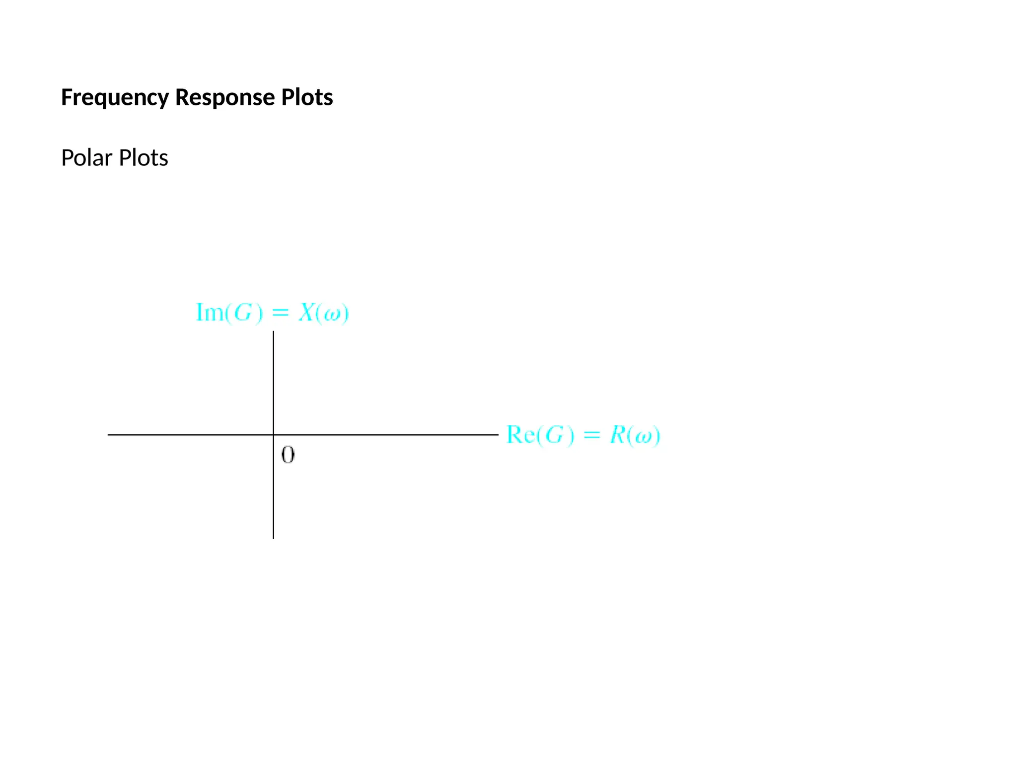
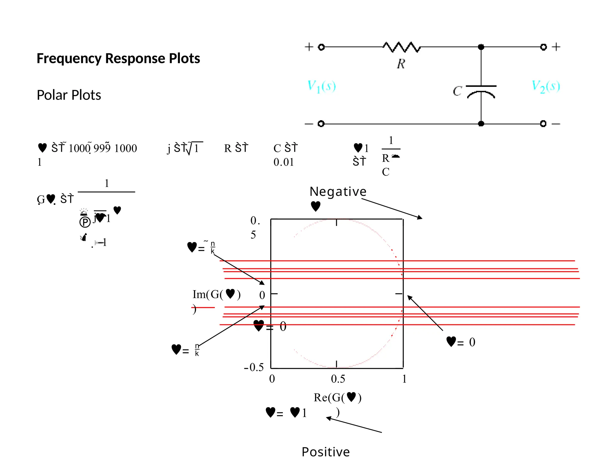
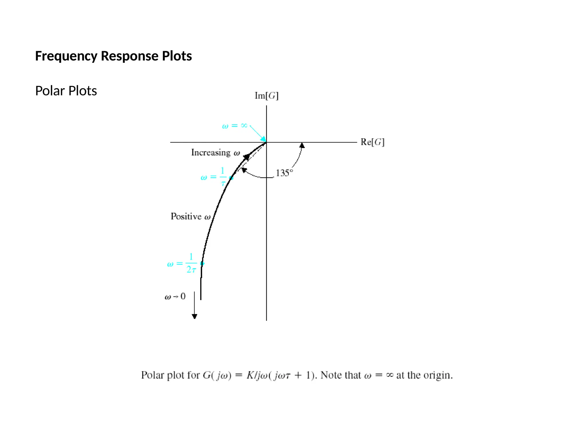
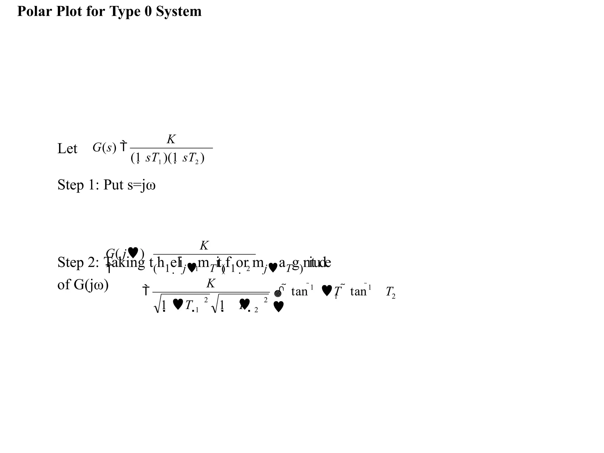
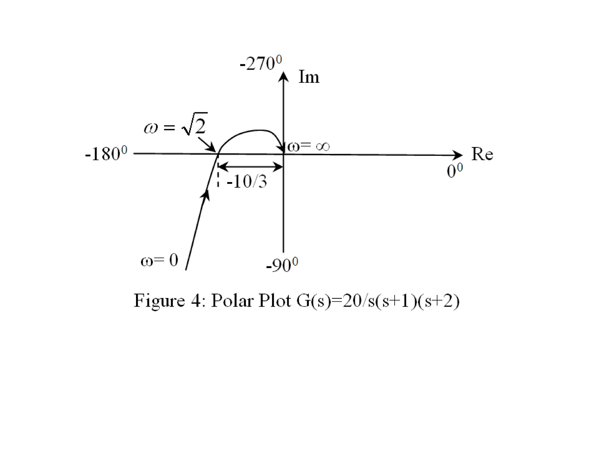
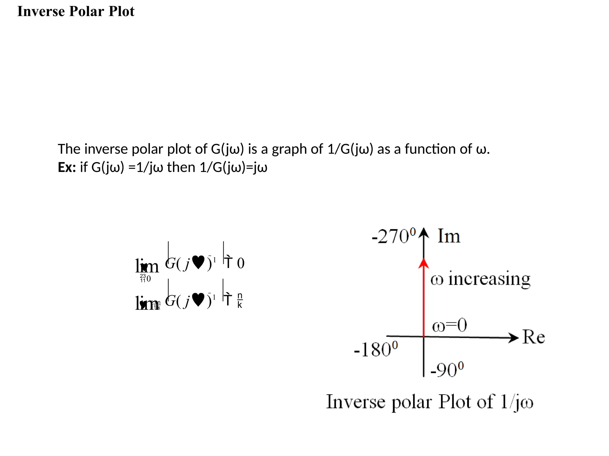
![Steps to draw Polar Plot
the real and imaginary parts
Step 6: Put Re [G(jω) ]=0, determine the frequency at which plot intersects the Im axis
and
)
Step 1: Determine the T.F G(s)
Step 2: Put s=jω in the G(s)
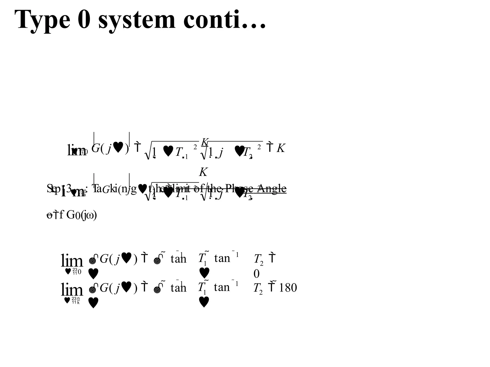
Step 3: At ω=0 & ω=∞ find by &
Step 4: At ω=0 & ω=∞ find by
Step 5: Rationalize the function G(jω) and
sep
&
Ga
r(a
t
je
G( j
)
lim G( j)
0 lim G( j)
lim
G( j)
calculate intersection value by putting the above calculated freque0ncy in
G(jω)
lim
G( j)
](https://image.slidesharecdn.com/pptcse1-250114082557-b9789d18/75/ppt-on-Control-system-engineering-1-pptx-315-2048.jpg)
![Steps to draw Polar Plot conti…
Step 7: Put Im [G(jω) ]=0, determine the frequency at which plot intersects the
real axis and calculate intersection value by putting the above calculated
frequency in G(jω)
Step 8: Sketch the Polar Plot with the help of above information](https://image.slidesharecdn.com/pptcse1-250114082557-b9789d18/75/ppt-on-Control-system-engineering-1-pptx-316-2048.jpg)
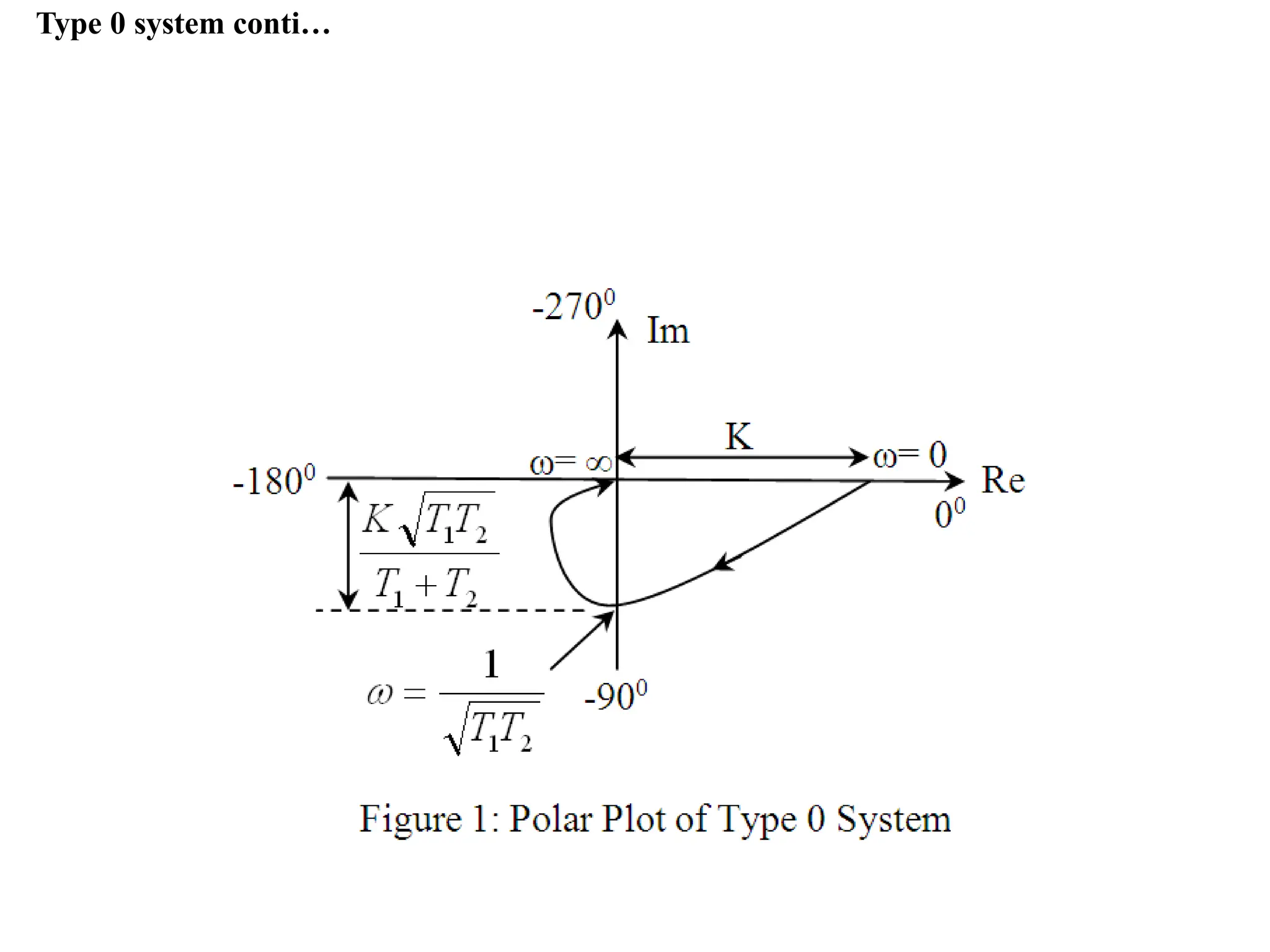
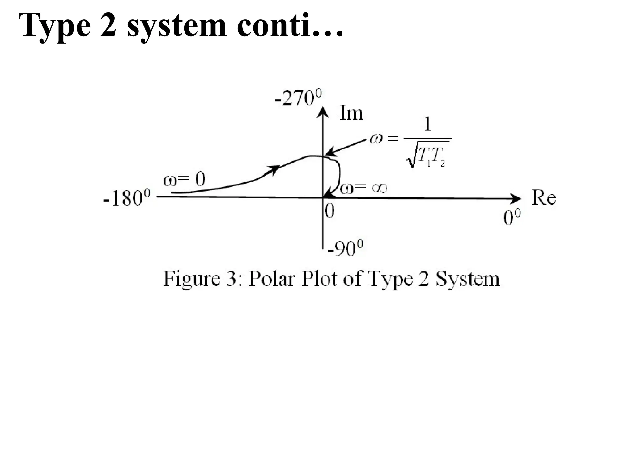
![Type 0 system conti…
Step 4: Separate the real and Im part of G(jω)
2 1 2
2 2 4
1
2 2
2 1 2
1
2 2 2 2 4
1 2
2
1 T T TT
K(T T )
j 1 2
1 T T TT
K (1
TT )
Step 5:GPu(tjRe)
[G(jω)]=0
G( j) 0 1800
900
T1 T2
T1T2
T1T2
1 2
1 2
2
2 2 4
2 2
1 2
0
1
So
When
&
G( j)
K
1
&
1
1 T T T
T
K (1 2
T T
)
T
T](https://image.slidesharecdn.com/pptcse1-250114082557-b9789d18/75/ppt-on-Control-system-engineering-1-pptx-319-2048.jpg)
![Type 0 system conti…
Step 6: Put Im [G(jω)]=0
2 1 2
2 2 2 2 4
0 G( j)
K00
G( j)
01800
1
So
When
K(T1 T2 )
0 0 &
1 T T TT](https://image.slidesharecdn.com/pptcse1-250114082557-b9789d18/75/ppt-on-Control-system-engineering-1-pptx-320-2048.jpg)
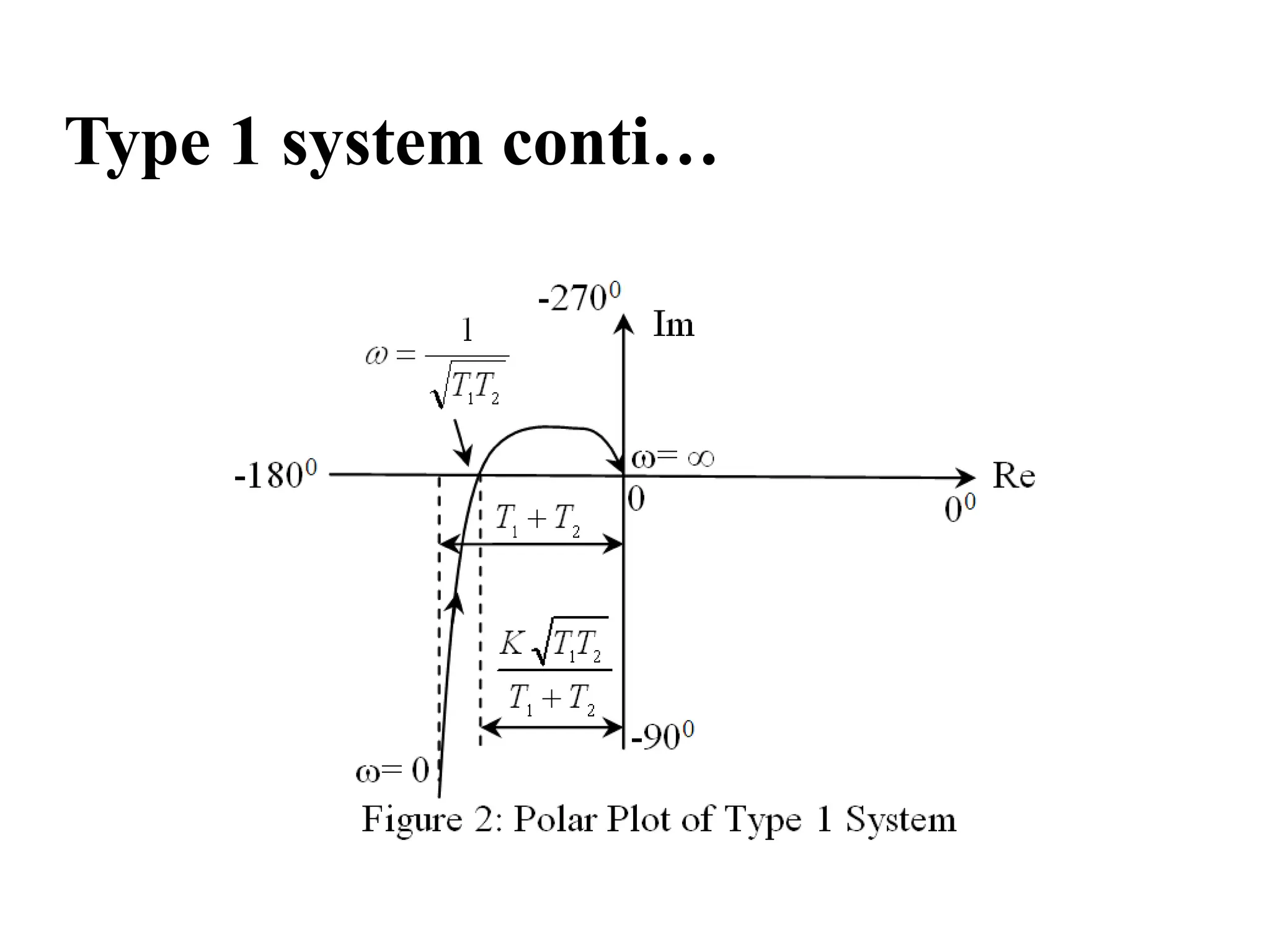
![Type 1 system conti…
Step 4: Separate the real and Im part of G(jω)
1 2
2 2 2
1 2
3 2
1 2
2
1
3 2 2 2 2
1 2
(T T 2
T T )
j(K 2
T T K )
j 1 2
(T T 2
T T )
K (T T )
Step 5: P
u
tGR(ej[
G)(j
ω
)
]
=
0
1 2
2
1
3 2 2 2 2
So at
G( j) 0
2700
(T T 2
T T )
K (T1 T2 )
0
](https://image.slidesharecdn.com/pptcse1-250114082557-b9789d18/75/ppt-on-Control-system-engineering-1-pptx-324-2048.jpg)
![Type 1 system conti…
Step 6: Put Im [G(jω)]=0
G( j)
00
0
0
T1 T2
T1T2
1 2
1 2
2
1 2
0
1
So When
3
(T 2
T 2
2
T 2
T 2
)
j(K 2
T T K )
G( j)
K
T1T2
1
1
&
T
T](https://image.slidesharecdn.com/pptcse1-250114082557-b9789d18/75/ppt-on-Control-system-engineering-1-pptx-325-2048.jpg)
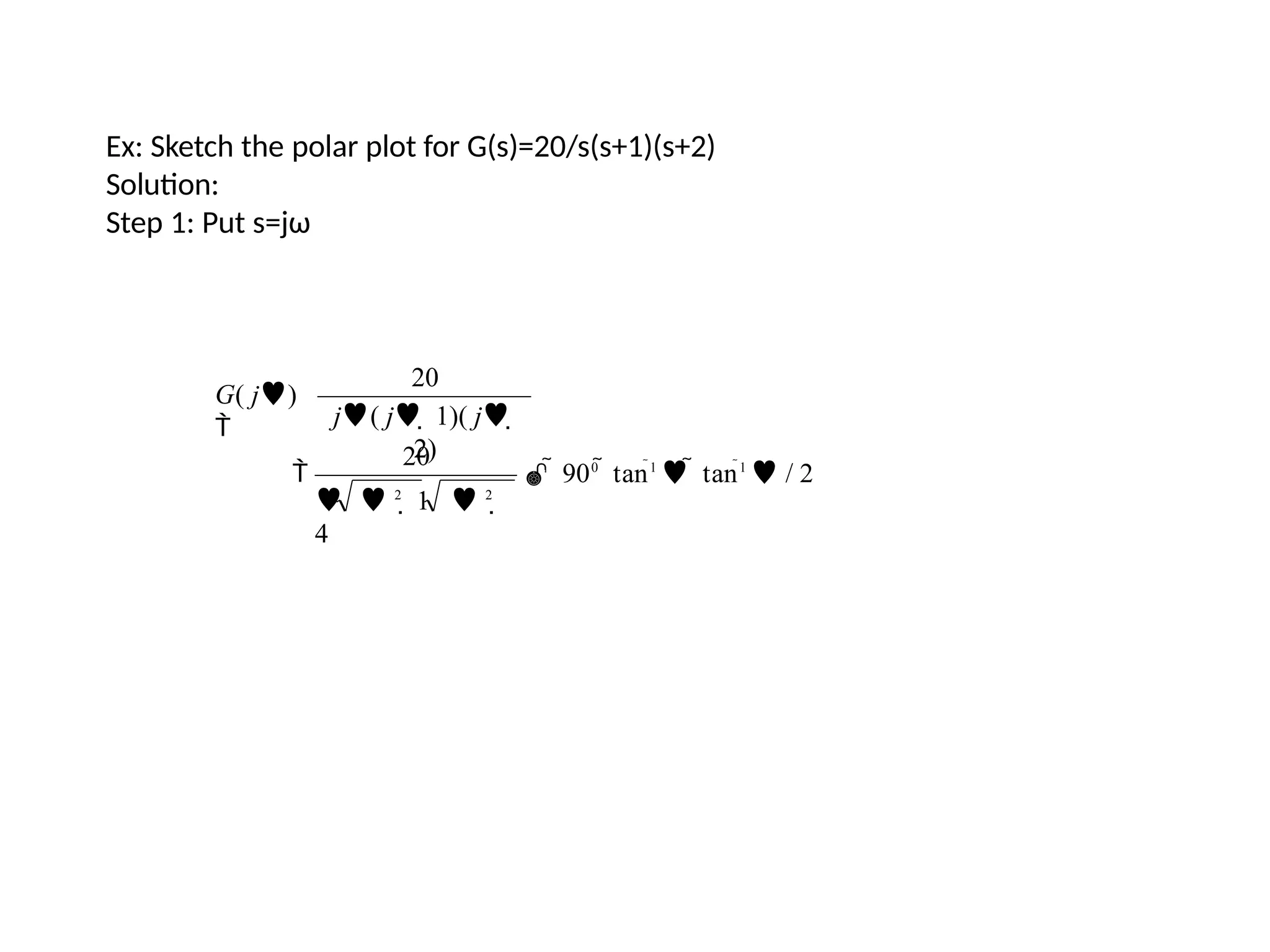
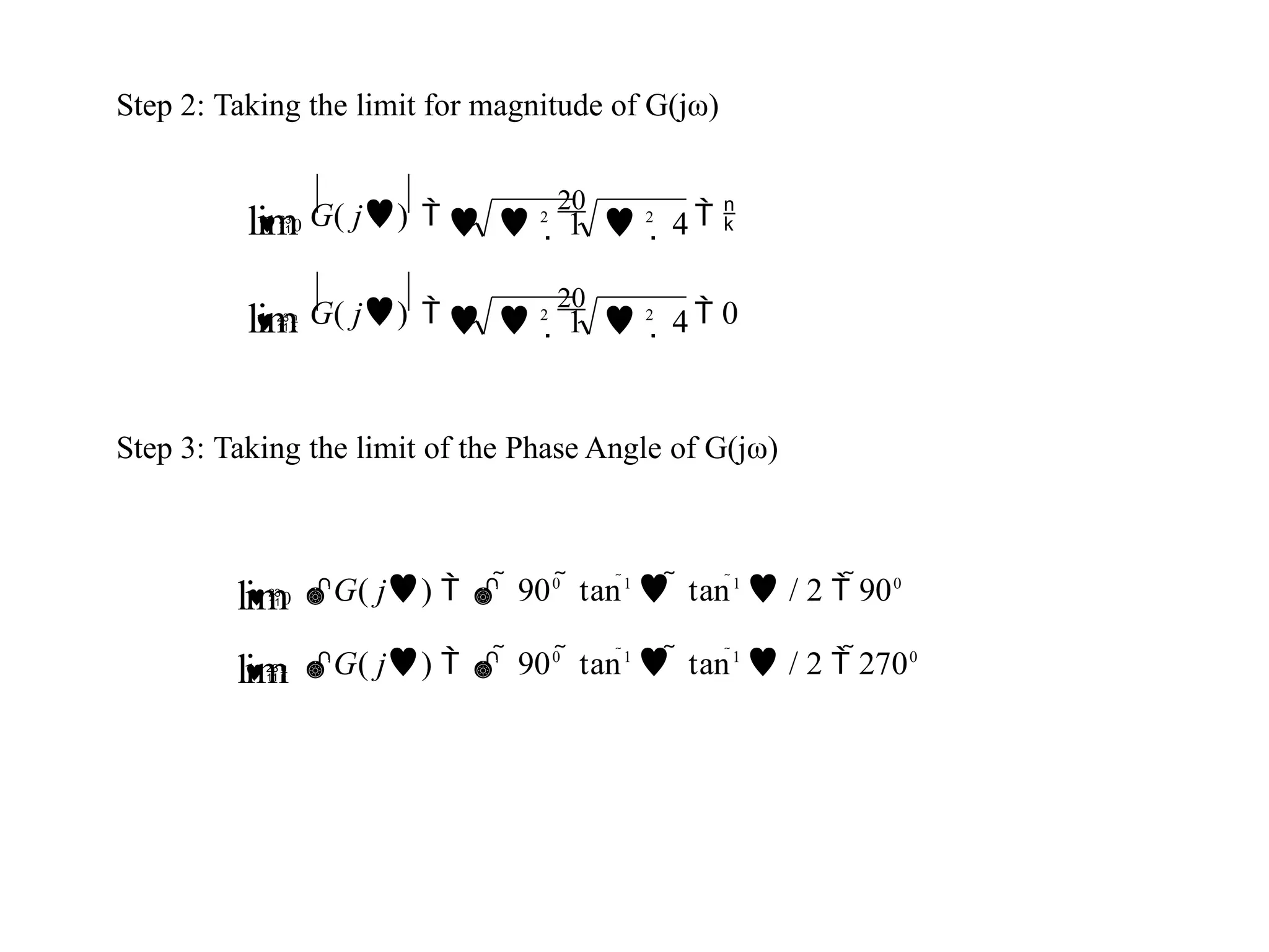
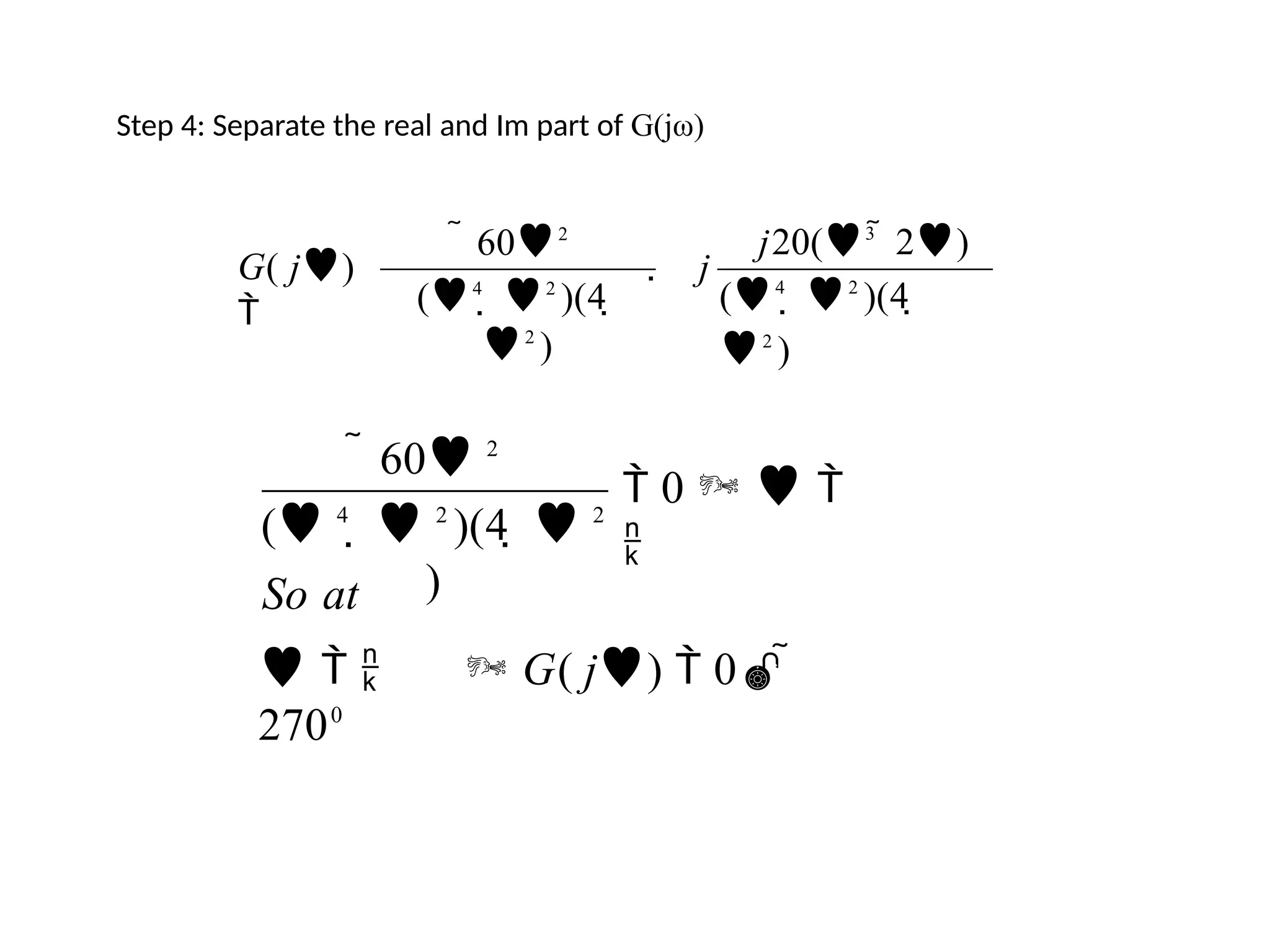
![Step 6: Put Im [G(jω)]=0
3
G( j)
000
2 G( j)
10
00
2 &
0
( 4
2
)(4 2
)
So for positivevalueof
j20( 3
2)
](https://image.slidesharecdn.com/pptcse1-250114082557-b9789d18/75/ppt-on-Control-system-engineering-1-pptx-333-2048.jpg)


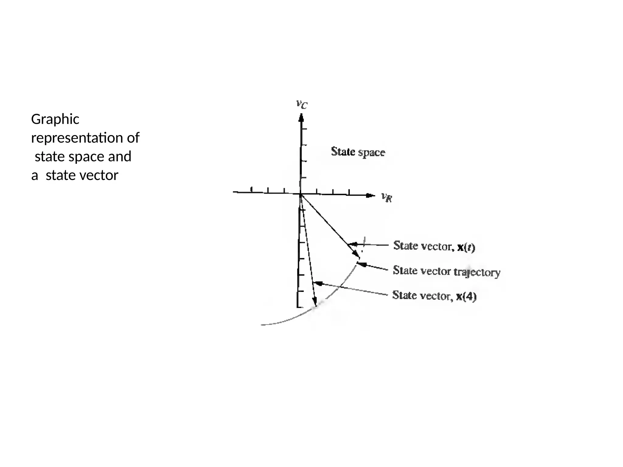
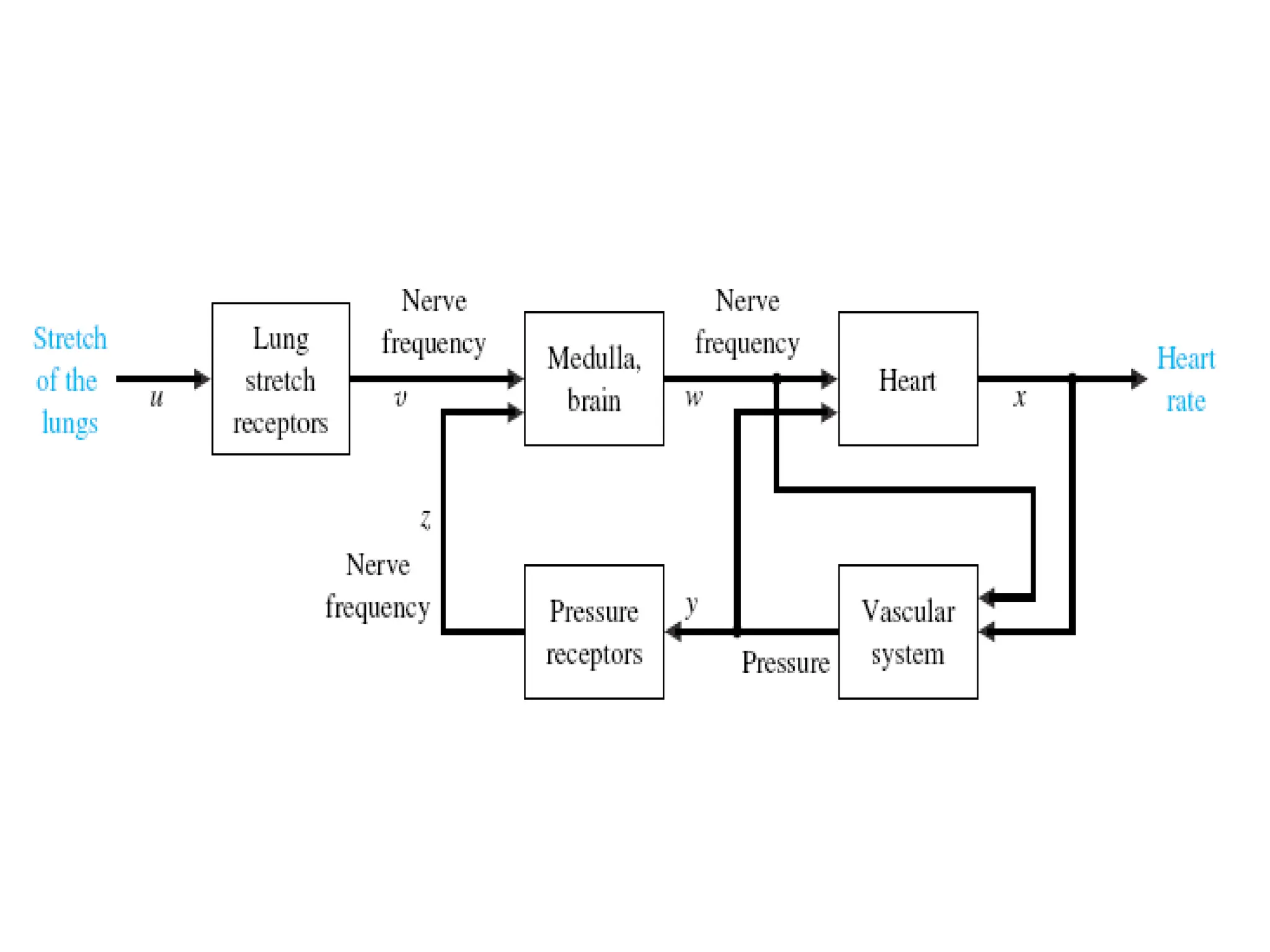
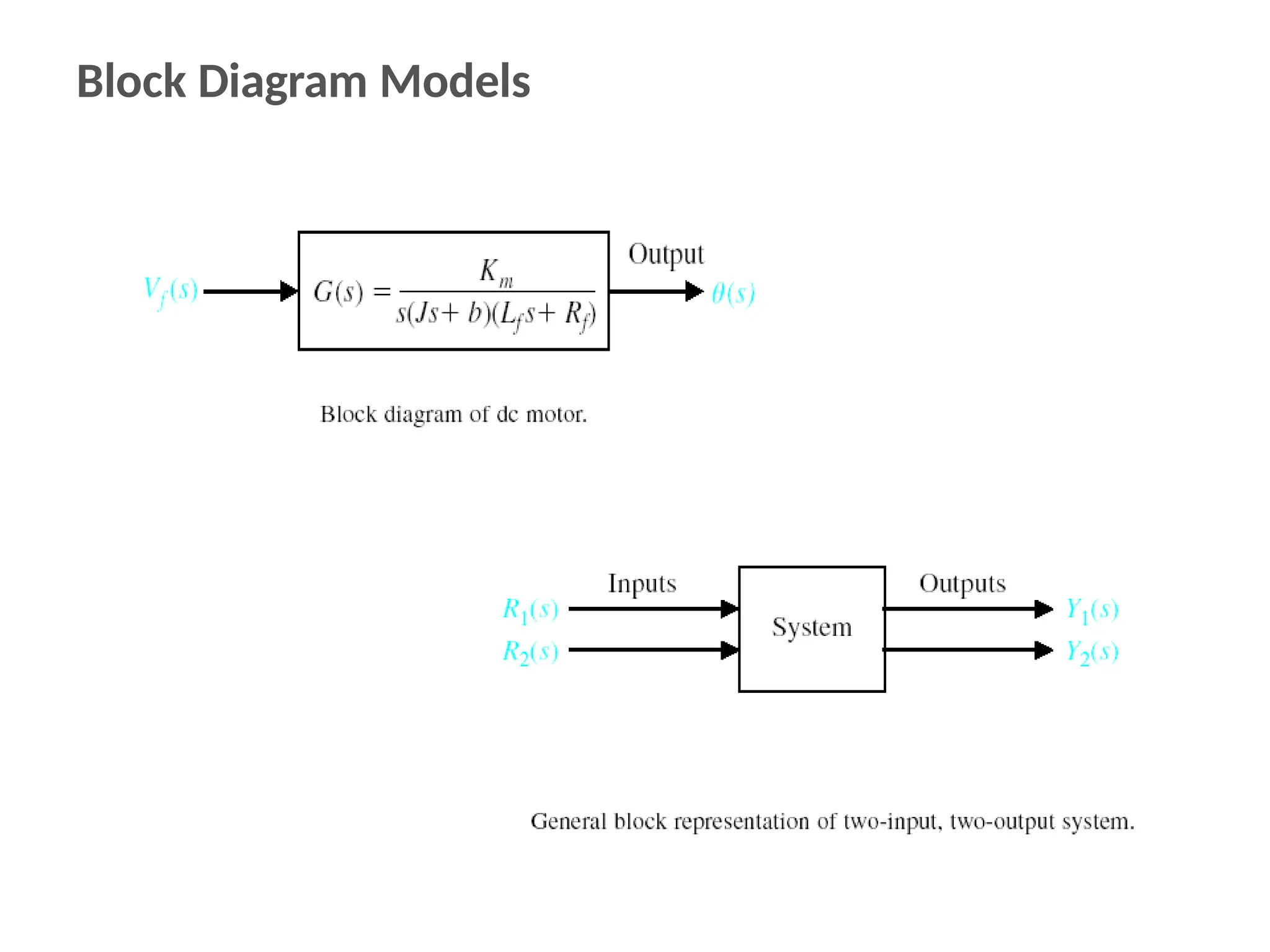
![For a dynamic system, the state of a system is described in terms of a set of state
variables
[x1 (t) x2 (t) … xn (t)]
The state variables are those variables that determine the future behavior of a
system when the present state of the system and the excitation signals are known.
Consider the system shown in Figure 1, where y1(t) and y2(t) are the output signals
and u1(t) and u2(t) are the input signals. A set of state variables [x1 x2 ... xn] for the
system shown in the figure is a set such that knowledge of the initial values of the
state variables [x1(t0) x2(t0) ... xn(t0)] at the initial time t0, and of the input signals
u1(t) and u2(t) for t˃=t0, suffices to determine the future values of the outputs and
state variables.
System
Input Signals
u1(t)
u2(t)
Output Signals
y1(t)
y2(t) System
u(t)
Input
x(0) Initial conditions
y(t)
Output
Figure 1. Dynamic system.](https://image.slidesharecdn.com/pptcse1-250114082557-b9789d18/75/ppt-on-Control-system-engineering-1-pptx-386-2048.jpg)
![In an actual system, there are several choices of a set of state variables that specify
the energy stored in a system and therefore adequately describe the dynamics of
the system.
The state variables of a system characterize the dynamic behavior of a system. The
engineer’s interest is primarily in physical, where the variables are voltages,
currents, velocities, positions, pressures, temperatures, and similar physical
variables.
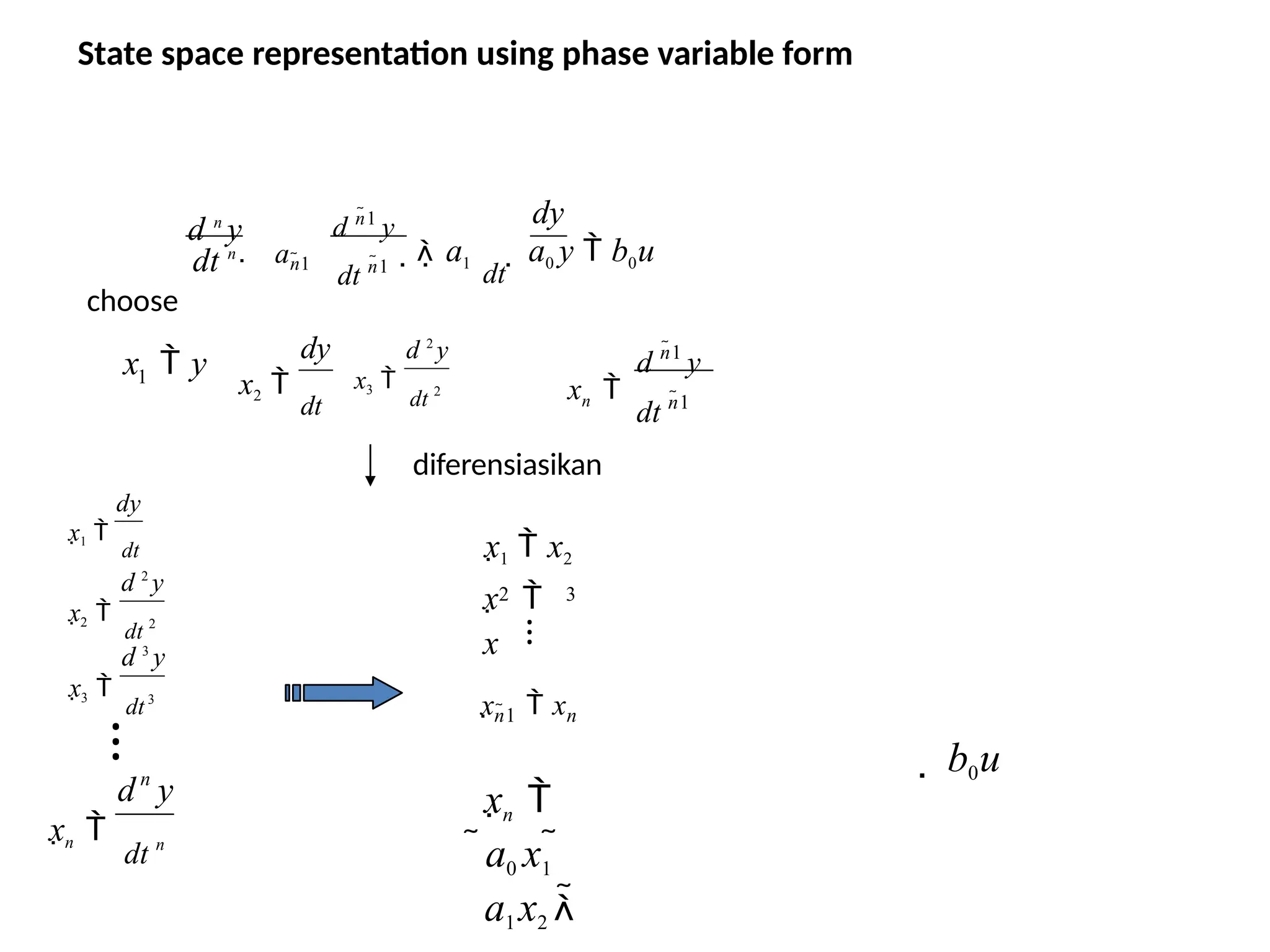
The State Differential Equation:
The state of a system is described by the set of first-order differential equations
written in terms of the state variables [x1 x2 ... xn]. These first-order differential
equations can be written in general form as
x 1 a1 1x1 a1 2x2 …a1n xn b1 1u1 b1m um
x 2 a 2 1x1 a 2 2x2 …a 2 n xn b2 1u1 b2 m um
⁝ an1x1 an 2 x2 …an n xn bn1u1 bn mum
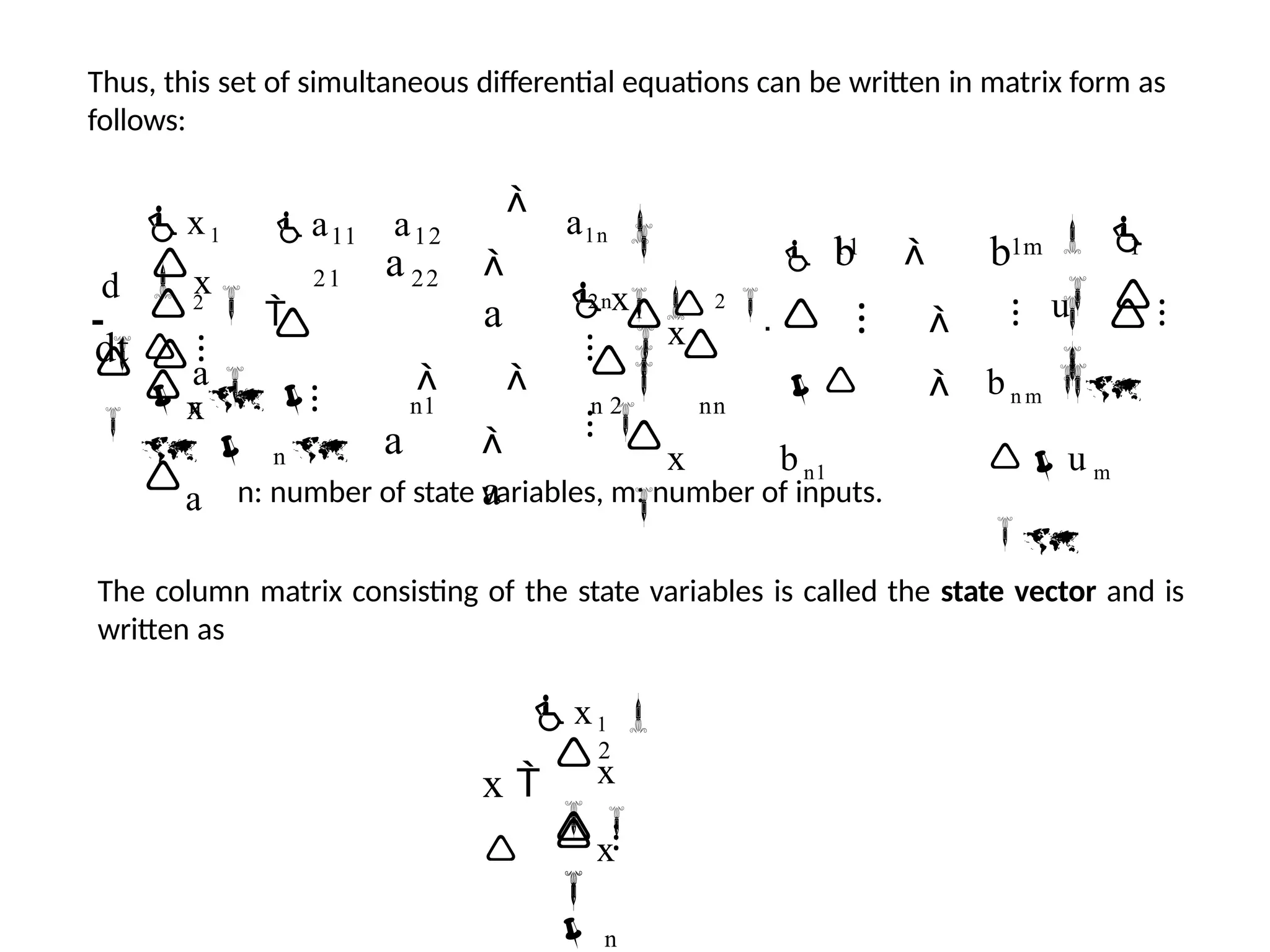
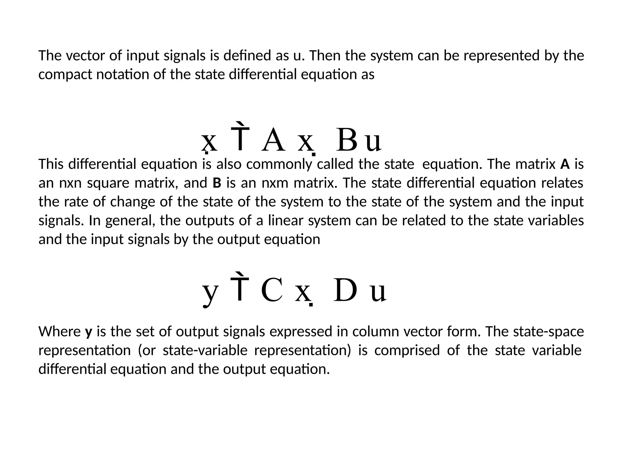
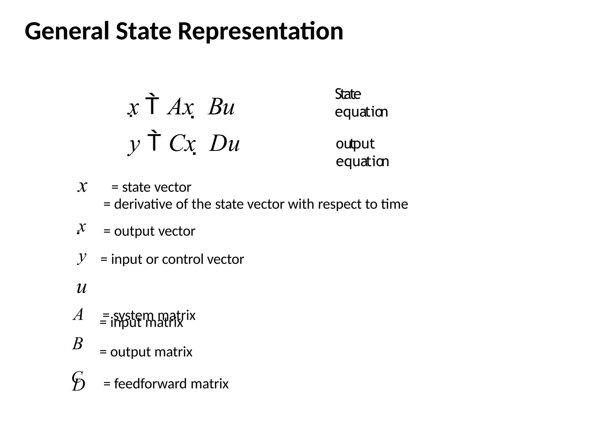
x n](https://image.slidesharecdn.com/pptcse1-250114082557-b9789d18/75/ppt-on-Control-system-engineering-1-pptx-387-2048.jpg)
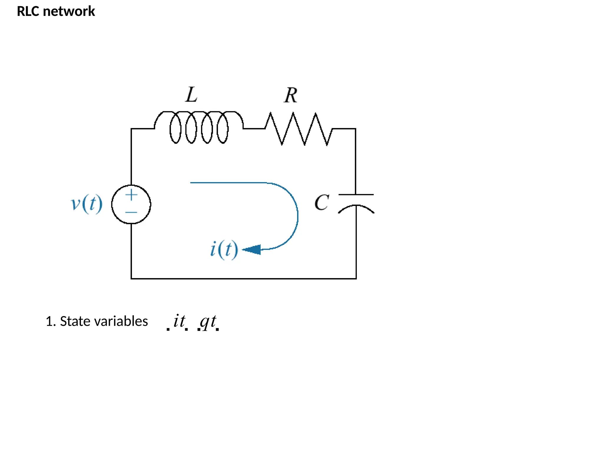
![AN EXAMPLE OF THE STATE VARİABLE CHARACTERİZATİON OF A SYSTEM
u(t)
Current
source
L
C
R
Vc
Vo
iL
ic
• The state of the system can be described in terms of a set of variables [x1 x2],
where x1 is the capacitor voltage vc(t) and x2 is equal to the inductor current iL(t).
This choice of state variables is intuitively satisfactory because the stored energy
of the network can be described in terms of these variables.](https://image.slidesharecdn.com/pptcse1-250114082557-b9789d18/75/ppt-on-Control-system-engineering-1-pptx-391-2048.jpg)
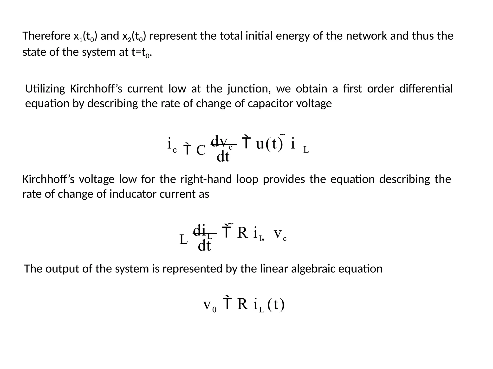
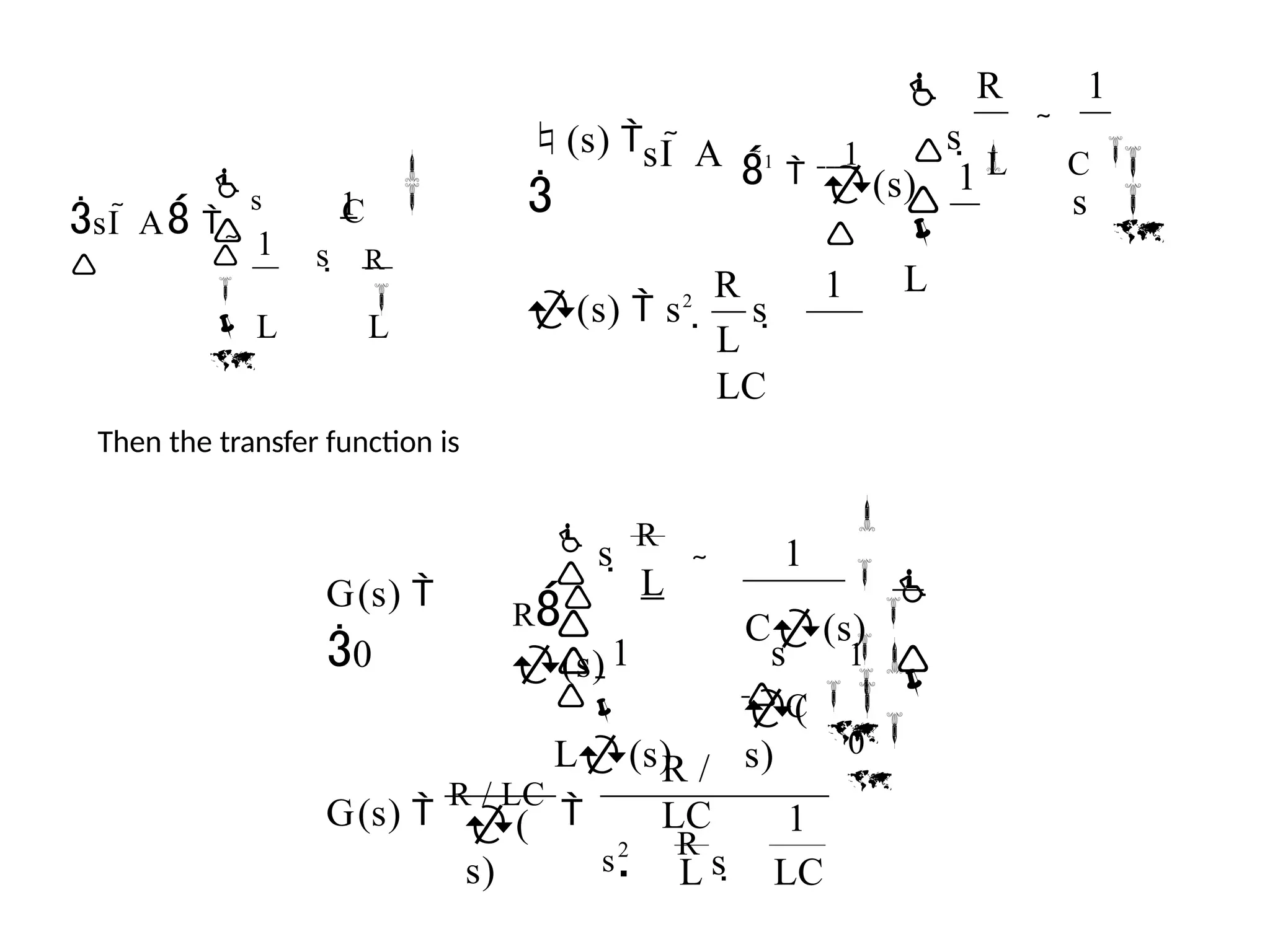
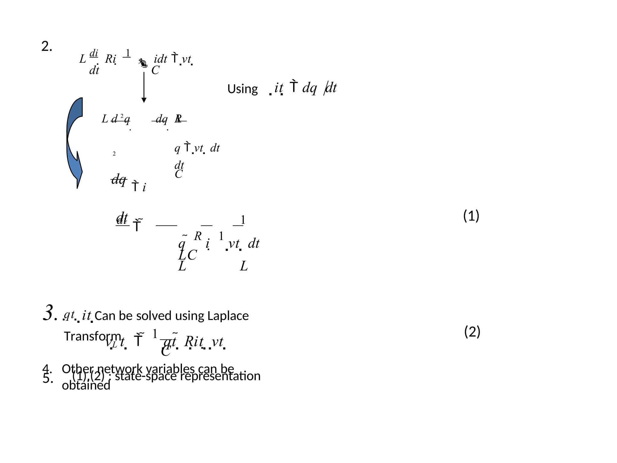
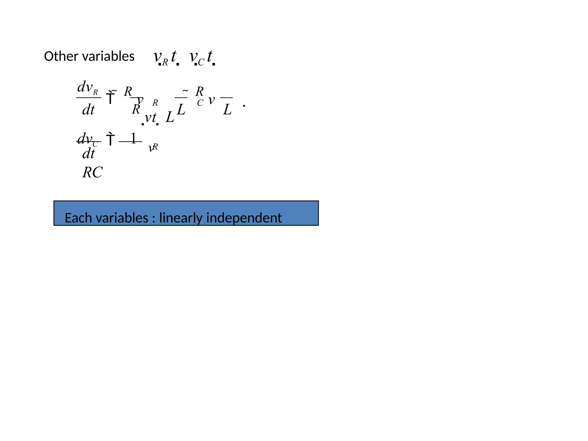
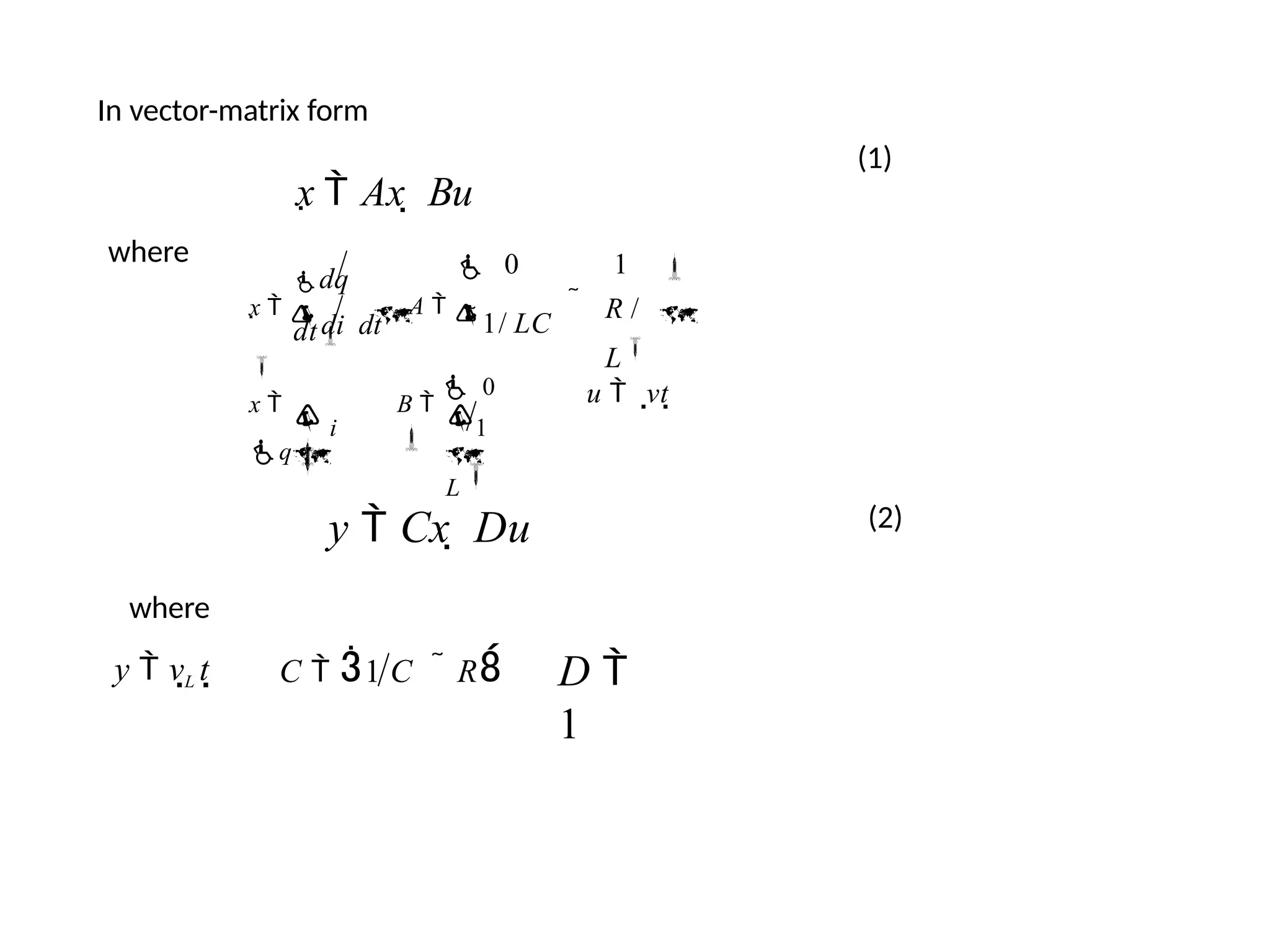
![We can write the equations as a set of two first order differential equations in terms
of the state variables x1 [vC(t)] and x2 [iL(t)] as follows:
2
1
dt
dx2
dx1 1
1
x2
u(t)
C
C
1
x
R
x dt L
L
L
C
dvc u(t) i
dt
diL
L R iL
vc dt
The output signal is then y1 (t) v0 (t) R x2
Utilizing the first-order differential equations and the initial conditions of the
network represented by [x1(t0) x2(t0)], we can determine the system’s future and its
output.
The state variables that describe a system are not a unique set, and several
alternative sets of state variables can be chosen. For the RLC circuit, we might
choose the set of state variables as the two voltages, vC(t) and vL(t).](https://image.slidesharecdn.com/pptcse1-250114082557-b9789d18/75/ppt-on-Control-system-engineering-1-pptx-393-2048.jpg)

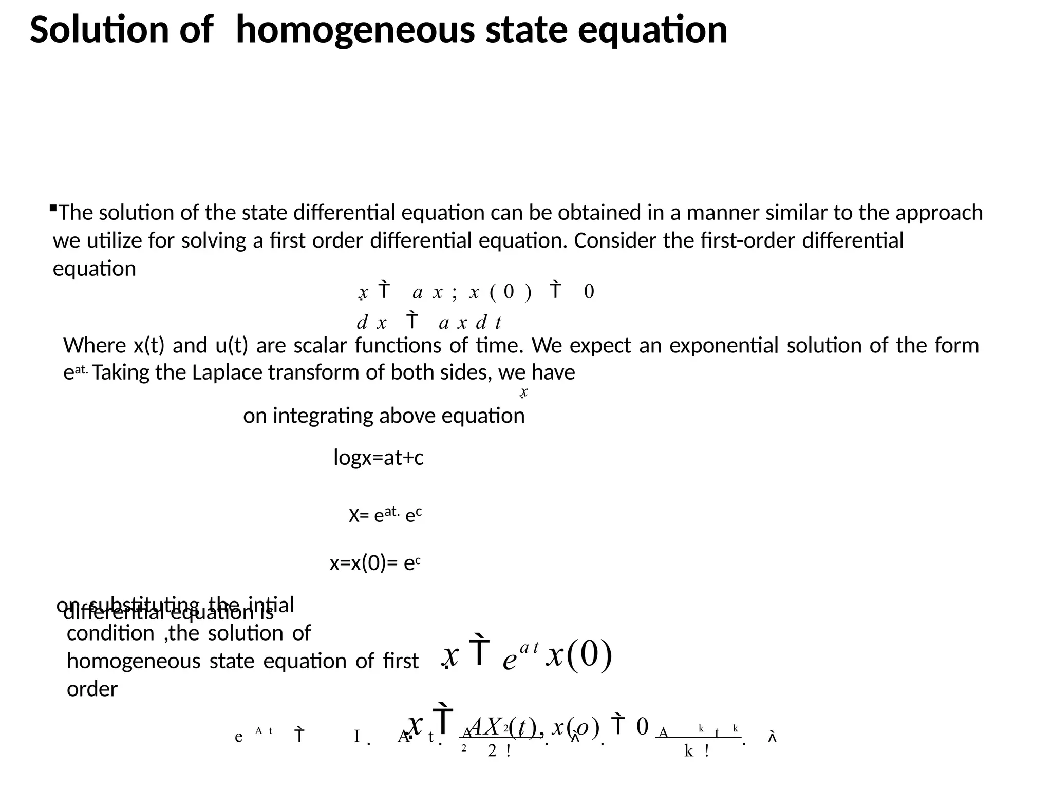
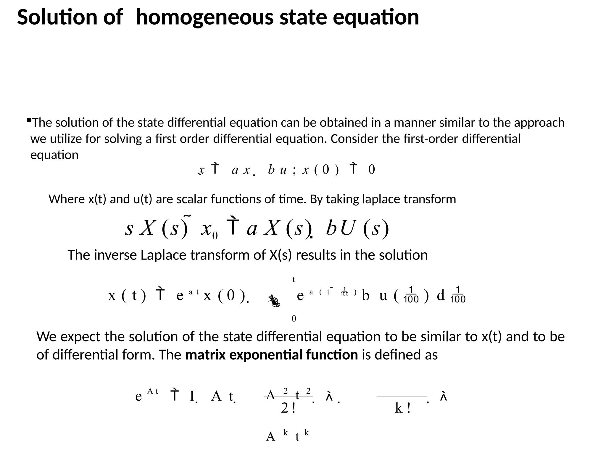
![which converges for all finite t and any A. Then the solution of the state
differential equation is found to be
t
x(t) eAt
x(0) eA ( t )
B u() d
0
X(s) sI A1
x(0) sI A1
B U(s)
where we note that [sI-A]-1=ϕ(s), which is the Laplace transform of ϕ(t)=eAt. The
matrix exponential function ϕ(t) describes the unforced response of the system
and is called the fundamental or state transition matrix.
t
x(t) (t) x(0) (t ) B u() d
0](https://image.slidesharecdn.com/pptcse1-250114082557-b9789d18/75/ppt-on-Control-system-engineering-1-pptx-412-2048.jpg)
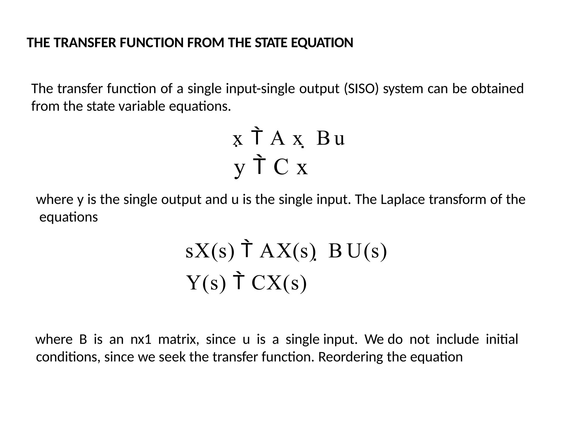
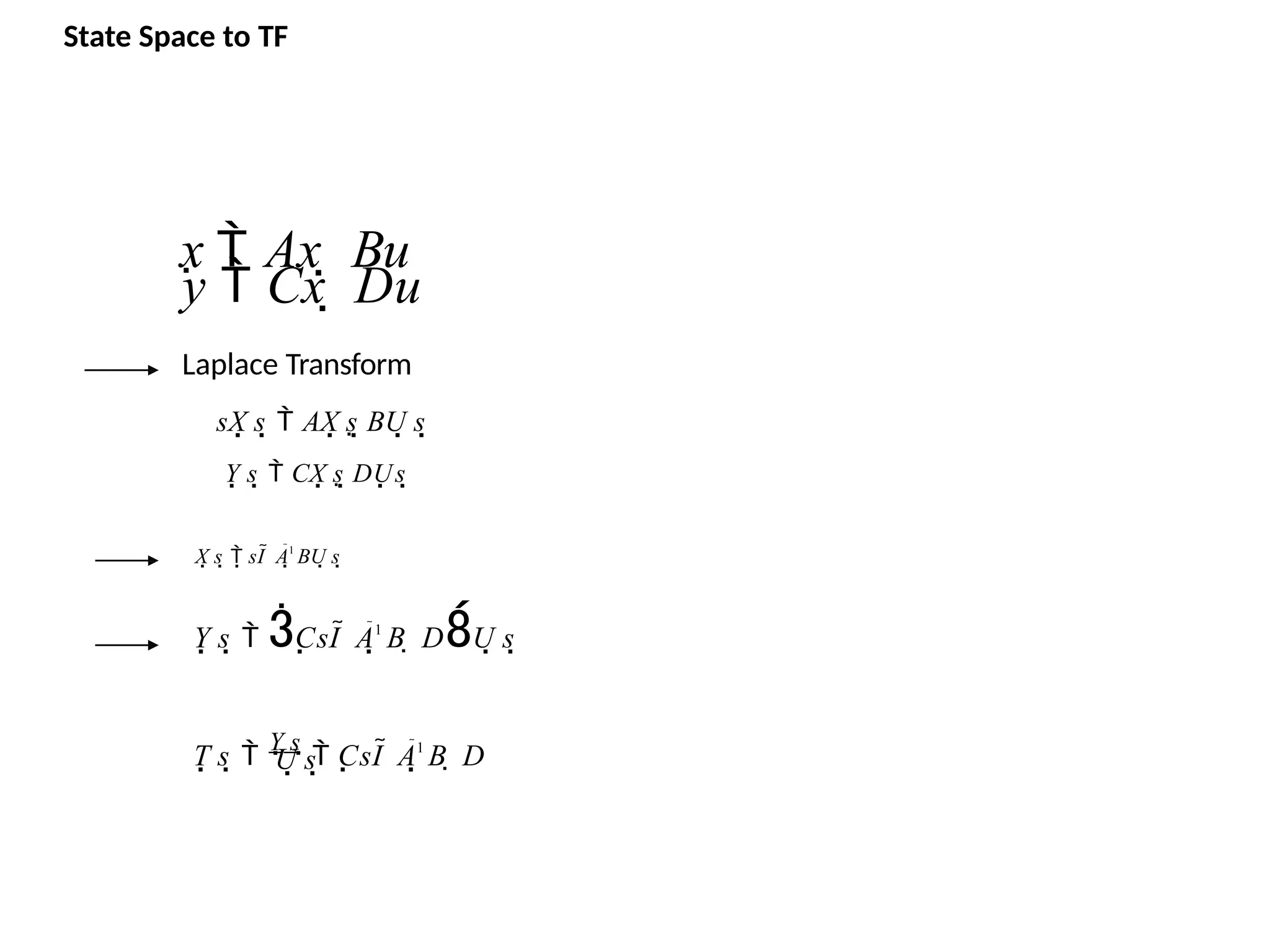
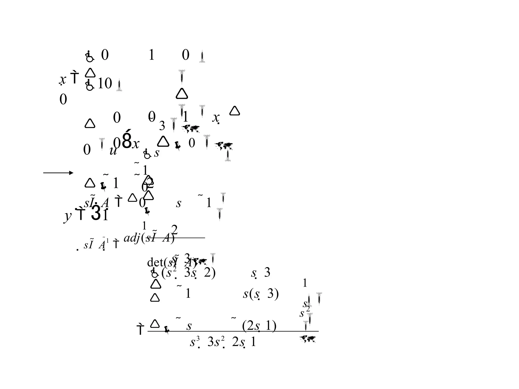
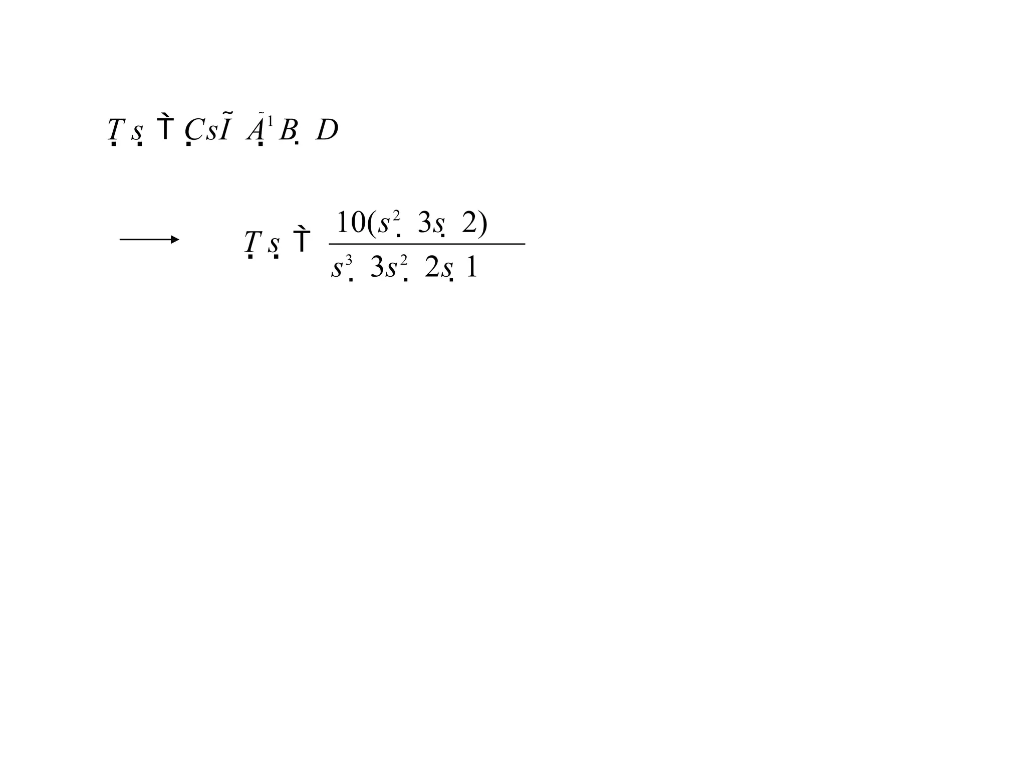
![[sI A]X(s) B U(s)
X(s) sI A1
BU(s)
(s)BU(s) Y(s) C(s)BU(s)
Therefore, the transfer function G(s)=Y(s)/U(s) is
G(s)
C(s)B
Example:
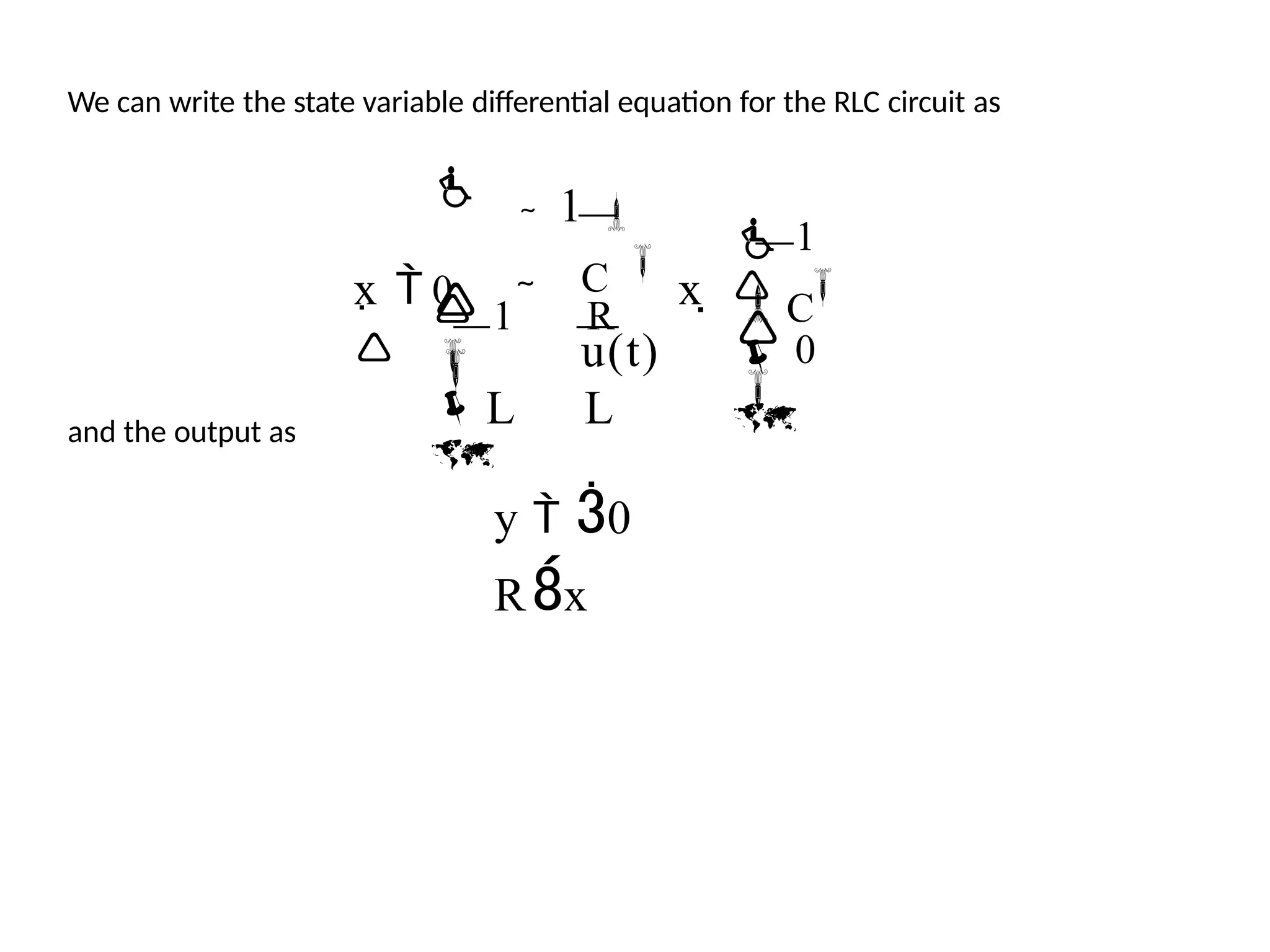
Determine the transfer function G(s)=Y(s)/U(s) for the RLC circuit as described by the
state differential function
, y 0
Rx
u
C
0
1
C
x
1 R
L L
1
0
x
](https://image.slidesharecdn.com/pptcse1-250114082557-b9789d18/75/ppt-on-Control-system-engineering-1-pptx-414-2048.jpg)