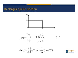
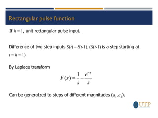
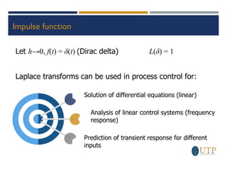
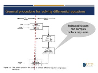
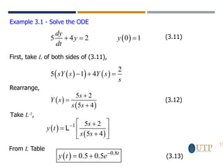
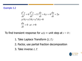
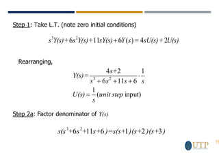
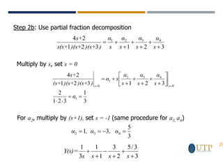
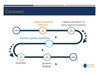
The document discusses the Laplace transform and its applications. It defines the Laplace transform and provides examples of transforms for typical functions like constants, step functions, exponentials, derivatives and trigonometric functions. It then discusses using Laplace transforms to solve differential equations by taking the transform of both sides of an equation and using properties to find the inverse transform and solution. The document also covers other Laplace transform properties like the final value theorem, initial value theorem and their applications in dynamic analysis.

1. Chapter 3:
Laplace Transform
BY
Assoc. Prof. Dr Marappagounder Ramasamy / Dr Serene Lock /
Dr Mohd Hilmi Noh / Dr Nurul Aini Amran
UNIVERSITI TEKNOLOGI PETRONAS (UTP)
CEB2083 PROCESS INSTRUMENTATION & CONTROL
MAY 2020 SEMESTER

2. Chapter Objectives
End of this chapter, you should be able to:
1. Use Laplace Transform of representative functions
2. Solve differential equations by Laplace Transform techniques
3. Explain other Laplace Transform properties
• Final value theorem
• Initial value theorem
• Time delay (translation in time)

3. Develop dynamic models of chemical processes
Design feedback control systems using modern IT tools
CLO1
CLO2
Select appropriate instruments for control systems
CLO3
Course learning outcomes

4. Laplace transform of representative functions


=
0
)
(
)]
(
[
)
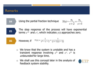
( dt
e
t
f
=
t
f
L
s
F -st
(3.1)
where F(s) is the symbol for the Laplace transform
s is a complex independent variable
f(t) is some function of time
The Laplace transform of a function f(t) is defined as

5. Transforms of some important functions
Constant function: f(t) = a
  s
a
s
a
e
s
a
dt
ae
=
a
L st
-st
=






−
−
=
−
=

−

 0
]
[
0
0
(3.2)

6. Transforms of some important functions
Step function
The unit step function is defined as





=
0
1
0
0
)
(
t
t
t
S (3.3)
The Laplace transform of the unit step function is
obtained with a = 1
s
t
S
L
1
)]
(
[ = (3.4)

7. Transforms of some important functions
Exponential Functions
bt
e−
, b > 0
  b
s
e
s
b
dt
e
dt
e
e
=
e
L t
s
b
t
s
b
-st
bt
bt
+
=
−
+
=
=

+
−

+
−

−
−


1
1
]
[
0
)
(
0
)
(
0
(3.5)

8. Transforms of some important functions
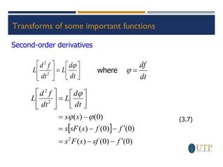
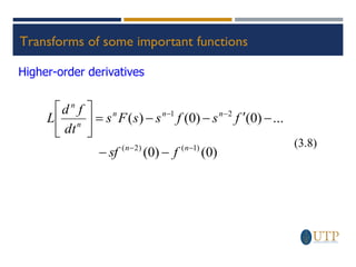
Derivatives
( ) ( )
)
0
(
)
(
)
0
(
]
[
)
(
)
(
]
[
0
0
0
f
s
sF
f
f
sL
e
t
f
sdt
e
t
f
dt
e
dt
df
=
dt
df
L
st
st
-st
−
=
−
=
+
= 



−
−

(3.6)
Usually define f(0) = 0

9. Transforms of some important functions
Second-order derivatives






=






dt
d
L
dt
f
d
L

2
2
where
dt
df
=

 
)
0
(
)
0
(
)
(
)
0
(
)
0
(
)
(
)
0
(
)
(
2
2
2
f
sf
s
F
s
f
f
s
sF
s
s
s
dt
d
L
dt
f
d
L

−
−
=

−
−
=
−
=






=









(3.7)

10. Transforms of some important functions
Higher-order derivatives
)
0
(
)
0
(
...
)
0
(
)
0
(
)
(
)
1
(
)
2
(
2
1
−
−
−
−
−
−
−

−
−
=






n
n
n
n
n
n
n
f
sf
f
s
f
s
s
F
s
dt
f
d
L
(3.8)

11. Transforms of some important functions
Trigonometric functions
Euler identity:
2
cos
t
j
t
j
e
e
t



−
+
=
cos sin
cos sin
1
j t
jwt
e t j t
e t j t
j

 
 
−
= +
= −
= −

12. Transforms of some important functions
Cosine function
 
2
2
2
2
2
1
1
1
2
1
2
cos









+
=






+
−
+
+
=








+
+
−
=





 +
=
−
s
s
s
j
s
j
s
j
s
j
s
e
e
L
t
L
t
j
t
j
Sine function
 
2
2
2
2
2
1
1
1
2
1
2
sin










+
=






+
+
−
+
=








+
−
−
=





 −
=
−
s
s
j
s
j
s
j
j
s
j
s
j
j
e
e
L
t
L
t
j
t
j
(3.9)

13. Rectangular pulse function
0
1 1
( ) (1 )
h
st hs
F s e dt e
h hs
− −
= = −










=
h
t
h
t
h
t
t
f
0
0
/
1
0
0
)
(
(3.10)

14. Rectangular pulse function
If h = 1, unit rectangular pulse input.
Difference of two step inputs S(t) – S(t-1). (S(t-1) is a step starting at
t = h = 1)
By Laplace transform
1
( )
s
e
F s
s s
−
= −
Can be generalized to steps of different magnitudes (a1, a2).

15. Impulse function
Let h→0, f(t) = δ(t) (Dirac delta) L(δ) = 1
Laplace transforms can be used in process control for:
Solution of differential equations (linear)
Analysis of linear control systems (frequency
response)
Prediction of transient response for different
inputs

16. General procedure for solving differential equations
Repeated factors
and complex
factors may arise.

17. 17
Example 3.1 - Solve the ODE
( )
5 4 2 0 1 (3-26)
dy
y y
dt
+ = = (3.11)
First, take L of both sides of (3.11),
( )
( ) ( )
2
5 1 4
sY s Y s
s
− + =
Rearrange,
( )
( )
5 2
(3-34)
5 4
s
Y s
s s
+
=
+
(3.12)
Take L-1,
( )
( )
1 5 2
5 4
s
y t
s s
−  
+
=  
+
 
L
From L Table
( ) 0.8
0.5 0.5 (3-37)
t
y t e−
= + (3.13)

18. 18
Example 3.2
0
0
0
0
0
0
2
4
6
11
6 2
2
3
3
at t=
dt
du
)=
(
y
)=
(
y
)=
y(
u
dt
du
y
dt
dy
dt
y
d
dt
y
d
=



+
=
+
+
+
To find transient response for u(t) = unit step at t > 0 :
1. Take Laplace Transform (L.T.)
2. Factor, use partial fraction decomposition
3. Take inverse L.T.

19. 19
Step 1: Take L.T. (note zero initial conditions)
3 2
6 11 6 ( ) 4 2
s Y(s)+ s Y(s)+ sY(s) Y s = sU(s)+ U(s)
+
Rearranging,
input)
(
1
1
6
11
6
2
4
2
3
step
unit
s
U(s)
s
s
s
s
s+
Y(s)=
=

+
+
+
Step 2a: Factor denominator of Y(s)
)
)(s+
)(s+
)=s(s+
s+
+
s
+
s(s 3
2
1
6
11
6 2
3

20. 20
Step 2b: Use partial fraction decomposition
3
2
1
3
2
1
2
4 4
3
2
1
+
+
+
+
+
+
=
s
α
s
α
s
α
s
α
)
)(s+
)(s+
s(s+
s+
Multiply by s, set s = 0
3
1
3
2
1
2
3
2
1
3
2
1
2
4
1
0
4
3
2
1
0
=
=








+
+
+
+
+
+
=
=
=
α
s
α
s
α
s
α
s
α
)
)(s+
)(s+
(s+
s+
s
s
For a2, multiply by (s+1), set s = -1 (same procedure for a3, a4)
3
5
3
1 4
3
2 =
−
=
= , α
, α
α
3
3
/
5
2
3
1
1
3
1
+
+
+
−
+
+
s
s
s
s
Y(s)=

21. 21
Step 3: Take inverse of L.T.
3
1
3
5
3
3
1 3
2
→

→
+
−
+ −
−
−
)
y(t
t
e
e
e
y(t)= t
t
t

22. Dynamic Analysis
Example 1:
2
2
3 4 1
s s
+ +
2
16
1.333 1
4 12
b
a
= = 
2 1
3 4 1 (3 1)( 1) 3( )( 1)
3
s s s s s s
+ + = + + = + +
Transforms to e-t/3, e-t (real roots) - (no oscillation)

23. Dynamic Analysis
2
2
1
s
s s
+
+ +
Example 2:
2
1
1
4 4
b
a
= 
2 3 3
1 ( 0.5 )( 0.5 )
2 2
s s s j s j
+ + = + + + −
Transforms to
0.5 0.5
3 3
sin , cos
2 2
t t
e t e t
− −
(oscillation)

24. Remarks
You can use this method on any order of ODE, limited only
by factoring of denominator polynomial (characteristic
equation).
Must use modified procedure for repeated roots, imaginary
roots.
One other useful feature of the Laplace transform is that
one can analyze the denominator of the transform to
determine its dynamic behavior. For example, if
2
3
1
2
+
+ s
s
Y(s)=
the denominator can be factored into (s+2)(s+1).
01
02
03

25. Remarks
05
06
04 Using the partial fraction technique
1
2
2
1
+
+
+ s
α
s
α
Y(s)=
The step response of the process will have exponential
terms e-2t and e-t, which indicates y(t) approaches zero.
However, if 𝑌(𝑠) =
1
𝑠2 − 𝑠 − 2
=
1
(𝑠 + 1)(𝑠 − 2)
o We know that the system is unstable and has a
transient response involving e2t and e-t. e2t is
unbounded for large time.
o We shall use this concept later in the analysis of
feedback system stability.

26. Other properties of L( ):
sY(s)
)=
y(
s 0
lim
→
 “offset”
Example 3: Step response
a
τs
a
τs
a
sY(s)
s
a
τs
Y(s)
s
=
+
+
=
+
=
→ 1
lim
1
1
1
0
offset (steady state error) is a.
Final value theorem:

27. Other properties of L( ):
Time-shift theorem: y(t)=0 t < 
sY(s)
y(t)=
s
t 
→
→
lim
lim
0
Example 4:
)
3
)(
2
)(
1
(
2
4
)
(
s+
s+
s+
s
s+
=
s
For Y
by initial value theorem: 0
)
0
( =
y
by final value theorem:
3
1
)
( =

y
Initial value theorem:

28. Conclusion!
FINISH
START
Laplace transform
definition
Laplace transform of
some typical functions
Inverse Laplace transforms
Examples Dynamic
Analysis