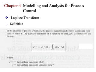
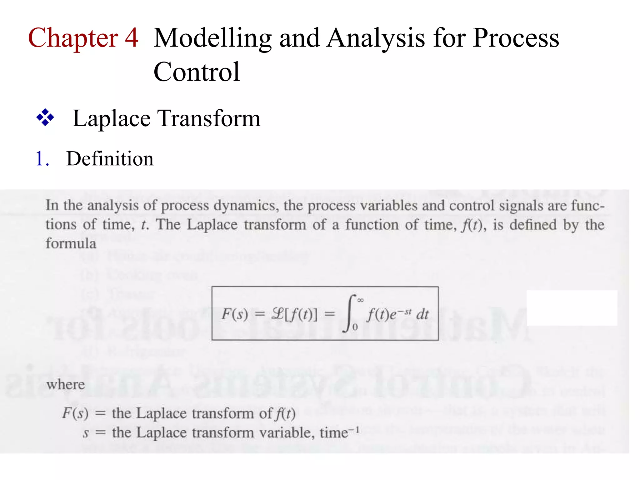
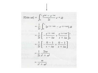
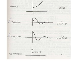
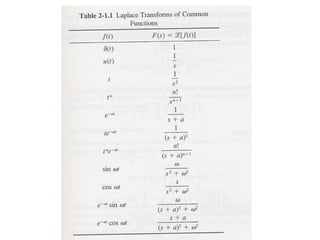
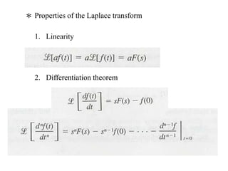
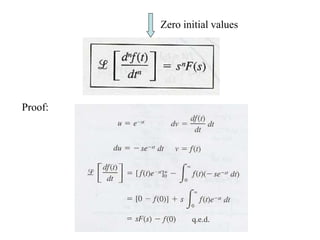
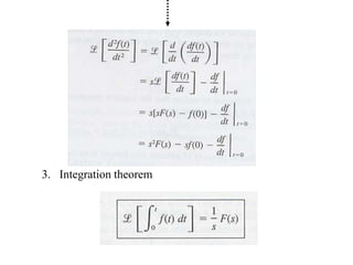
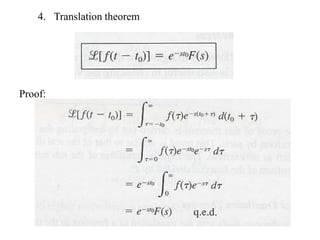
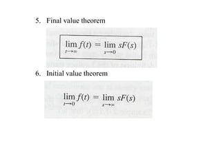
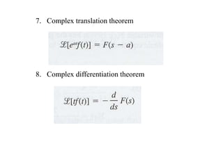
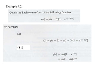
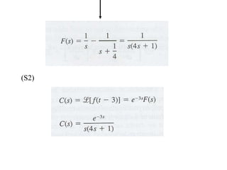
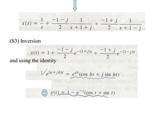
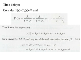
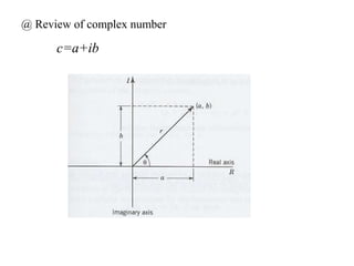
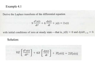
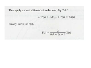
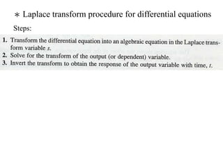
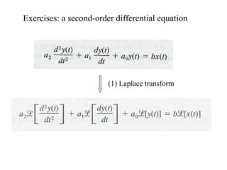
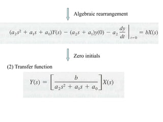
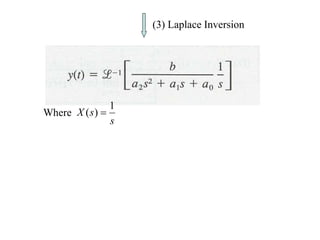
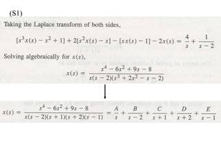
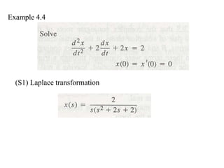
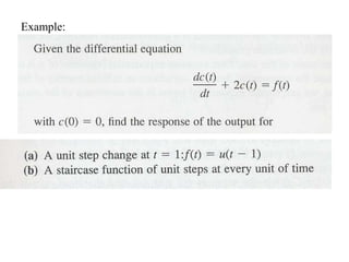
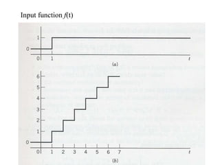
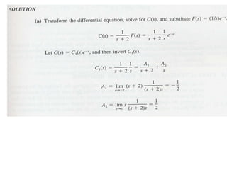
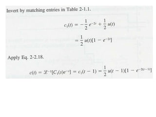
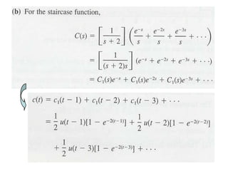
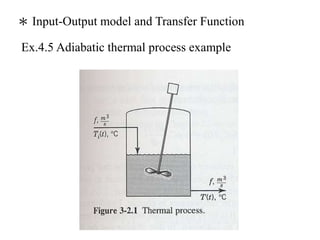
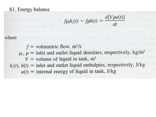
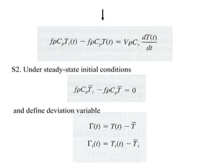
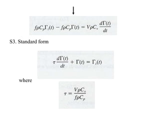
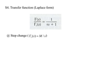
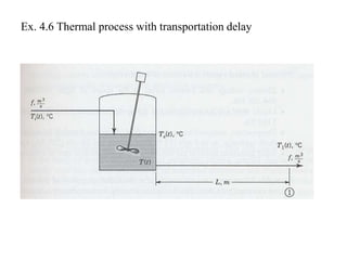
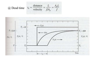
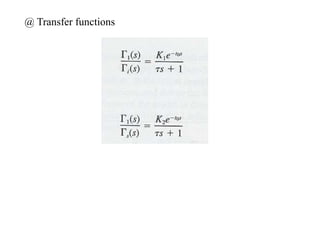
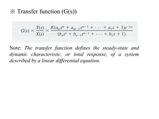
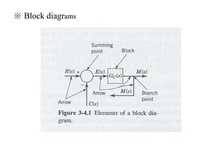
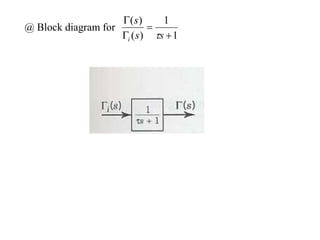
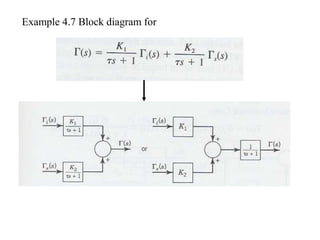
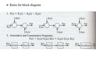
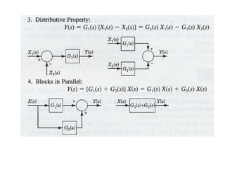
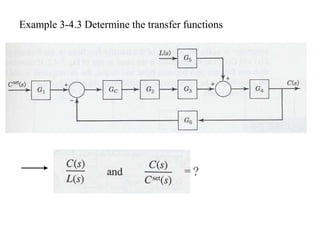
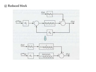
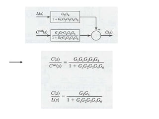
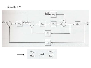
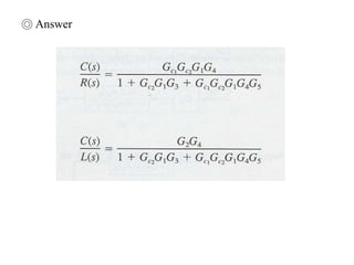
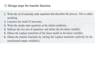
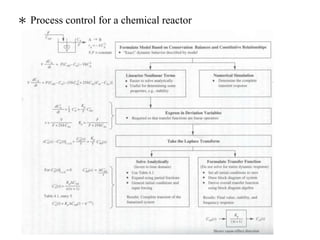
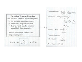
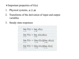
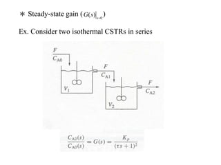
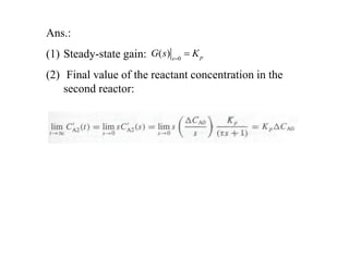
The document discusses Laplace transforms and their properties and applications in modeling dynamic systems. It covers: 1) Definition of the Laplace transform and properties including linearity, differentiation, integration, and translations. 2) Using Laplace transforms to derive transfer functions from differential equations describing dynamic systems. 3) The meaning and uses of transfer functions to characterize steady-state gains and dynamic responses of systems. 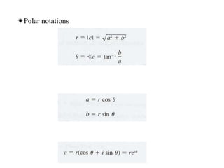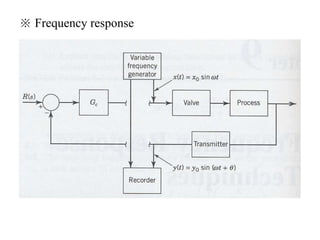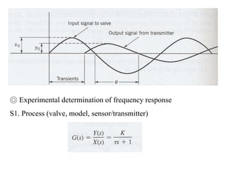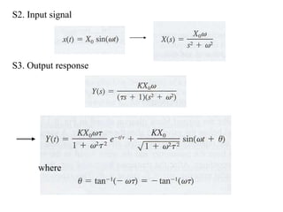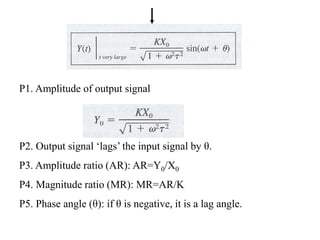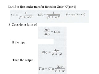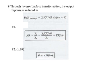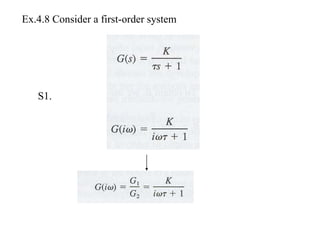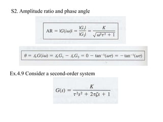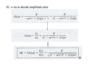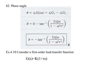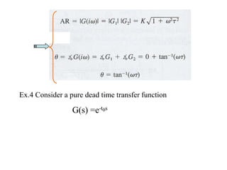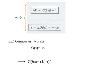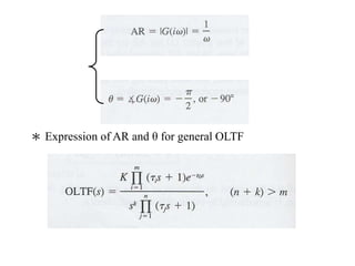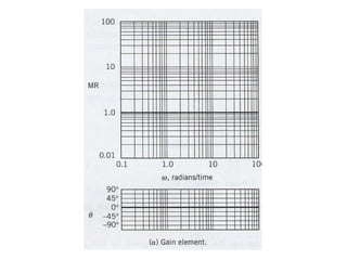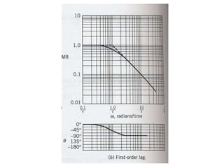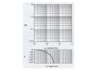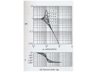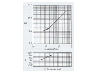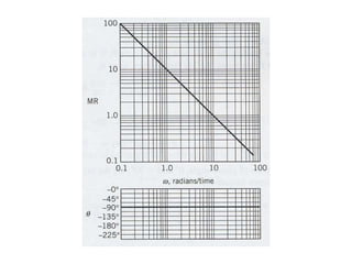4) Determining amplitude ratios and phase angles from transfer functions to analyze frequency responses. 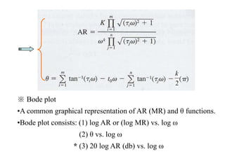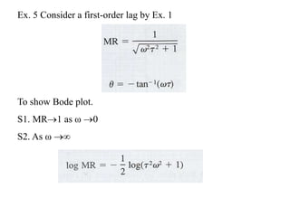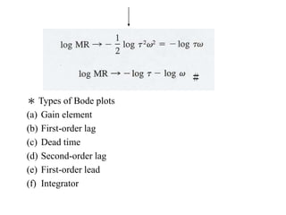5) Creating Bode plots to graphically represent frequency responses on logarithmic scales.

1.  Laplace Transform
1. Definition
Chapter 4 Modelling and Analysis for Process
Control

2. 2. Input signals

4. (c) A unit impulse function (Dirac delta function)

11. ＊ Properties of the Laplace transform
1. Linearity
2. Differentiation theorem

12. Zero initial values
Proof:

13. 3. Integration theorem

14. 4. Translation theorem
Proof:

17. 5. Final value theorem
6. Initial value theorem

18. 7. Complex translation theorem
8. Complex differentiation theorem

19. Example 4.1
Solution:

21. Example 4.2
(S1)

22. (S2)

23. ＊ Laplace transform procedure for differential equations
Steps:

24. Exercises: a second-order differential equation
(1) Laplace transform

25. Algebraic rearrangement
(2) Transfer function
Zero initials

26. (3) Laplace Inversion
Where
s
s
X
1
)
( 

27. Inversion method: Partial fractions expansion (pp.931)
(i) Fraction of denominator
and

28. (ii) Partial fractions
where

29. (iii) Inversion
＊ Repeated roots
If r1=r2, the expansion is carried out as

30. where
Inversion

31. ＊ Repeated roots for m times
If the expansion is carried out as

32. and

36. and A3=2 as (a) case.

37. The step response:
Example 4.3

38. (S1)

39. (S3) Find coefficients
s=0
Inversion

40. Example 4.4
(S1) Laplace transformation

41. (S2) Find coefficients
s=0
s=1-j
s=-1+j

42. (S3) Inversion
and using the identity

43. Time delays:
Consider Y(s)=Y1(s)e-st0 and

44. Example:

45. Input function f(t)

49. ＊ Input-Output model and Transfer Function
Ex.4.5 Adiabatic thermal process example

50. S1. Energy balance

51. S2. Under steady-state initial conditions
and define deviation variable

52. S3. Standard form
where

53. S4. Transfer function (Laplace form)
@ Step change ( )
s
M
s
i /
)
( 


55. ＊ Non-adiabatic thermal process example
S1. model
S2. Under deviation variables, the standard form

56. where

57. S3. Laplace form
@ Transfer functions

58. Ex. 4.6 Thermal process with transportation delay

59. @ Dead time

60. @ Transfer functions

61. ※ Transfer function (G(s))
Note: The transfer function defines the steady-state and
dynamic characteristic, or total response, of a system
described by a linear differential equation.

62. ＊Important properties of G(s)
1. Physical systems,
2. Transforms of the derivation of input and output
variables
3. Steady state responses
m
n 

63. ＊ Steady-state gain ( )
Ex. Consider two isothermal CSTRs in series
0
( ) s
G s 

64. Ans.:
(1) Steady-state gain:
(2) Final value of the reactant concentration in the
second reactor:
0
( ) p
s
G s K



65. ※ Block diagrams

66. @ Block diagram for
1
1
)
(
)
(




s
s
s
i 

67. Example 4.7 Block diagram for

68. ＊ Rules for block diagram

71. Example 4.8 Determine the transfer functions

73. Solution:
◎
◎

74. Example 3-4.3 Determine the transfer functions
=？

75. @ Reduced block

77. Example 4.9
=？

78. ◎ Answer

79. ◎ Design steps for transfer function

80. @ Review of complex number
c=a+ib

81. Polar notations

82. ※ Frequency response

83. ◎ Experimental determination of frequency response
S1. Process (valve, model, sensor/transmitter)

84. S2. Input signal
S3. Output response
where

85. P1. Amplitude of output signal
P2. Output signal ‘lags’ the input signal by θ.
P3. Amplitude ratio (AR): AR=Y0/X0
P4. Magnitude ratio (MR): MR=AR/K
P5. Phase angle (θ): if θ is negative, it is a lag angle.

86. Ex.4.7 A first-order transfer function G(s)=K/(τs+1)
＊ Consider a form of
If the input is set as
Then the output

87. ＊Through inverse Laplace transformation, the output
response is reduced as
P1.
P2. (p.69)

88. Ex.4.8 Consider a first-order system
S1.

89. S2. Amplitude ratio and phase angle
Ex.4.9 Consider a second-order system

90. S1. s=iω to decide amplitude ratio
＃

91. S2. Phase angle
＃
Ex.4.10 Consider a first-order lead transfer function
G(s)=K(1+τs)

92. Ex.4 Consider a pure dead time transfer function
G(s) =e-t0s

93. Ex.5 Consider an integrator
G(s)=1/s
G(i)=-(1/ )i

94. ＊ Expression of AR and θ for general OLTF

95. ※ Bode plot
•A common graphical representation of AR (MR) and θ functions.
•Bode plot consists: (1) log AR or (log MR) vs. log ω
(2) θ vs. log ω
* (3) 20 log AR (db) vs. log ω
2
k

96. Ex. 5 Consider a first-order lag by Ex. 1
To show Bode plot.
S1. MR1 as ω 0
S2. As ω 

97. ＃
＊ Types of Bode plots
(a) Gain element
(b) First-order lag
(c) Dead time
(d) Second-order lag
(e) First-order lead
(f) Integrator

104. ＊ Process control for a chemical reactor

106. Homework 2#
(1) Q4.6
(2) Q4.10
(3) Q4.16
(4) Q4.18 (※Difficulty)