This document contains lecture notes on introduction to control systems from Dr. Huynh Thai Hoang of Ho Chi Minh City University of Technology. The notes cover mathematical models of continuous control systems, including the concept of transfer functions. Chapter 2 discusses different mathematical models like transfer functions, block diagram algebra, signal flow graphs, and state space equations. It also covers linearized models of nonlinear systems.


![Block diagram algebra
Block diagram algebra –
– Example 1 (cont’)
Example 1 (cont’)
I h i h i i c d d
‘ Interchanging the summing points c and d,
Eliminating GA(s)=[G3(s)//G4(s)]
Y(s)
)
(
)
(
)
( 4
3 s
G
s
G
s
GA −
=
20 September 2011 48
© H. T. Hoang - www4.hcmut.edu.vn/~hthoang/](https://image.slidesharecdn.com/introctrlsyschapter2-221125011933-bf3748c7/85/IntroCtrlSys_Chapter2-pdf-48-320.jpg)
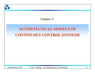
![Block diagram algebra
Block diagram algebra –
– Example 1 (cont’)
Example 1 (cont’)
‘ G ( ) [G ( ) // unity block]
‘ GB(s)=[G1(s) // unity block] ,
GC (s)= feedback loop[G2(s),GA(s)]:
Y( )
)
(
1
)
( s
G
s
G +
=
Y(s)
)
(
1
)
( 1 s
G
s
GB +
=
)]
(
)
(
) [
(
1
)
(
)
(
)
(
1
)
(
)
( 2
2
s
G
s
G
s
G
s
G
s
G
s
G
s
G
s
GC
−
+
=
+
=
)]
(
)
(
).[
(
1
)
(
).
(
1 4
3
2
2 s
G
s
G
s
G
s
G
s
G A +
+
‘ Equivalent transfer function of the system:
)
(
).
(
)
( s
G
s
G
s
G C
B
eq =
)
(
)].
(
1
[
)
( 2
1 s
G
s
G
s
G
+
=
20 September 2011 49
)]
(
)
(
).[
(
1
)
(
4
3
2 s
G
s
G
s
G
s
Geq
−
+
=
© H. T. Hoang - www4.hcmut.edu.vn/~hthoang/](https://image.slidesharecdn.com/introctrlsyschapter2-221125011933-bf3748c7/85/IntroCtrlSys_Chapter2-pdf-49-320.jpg)


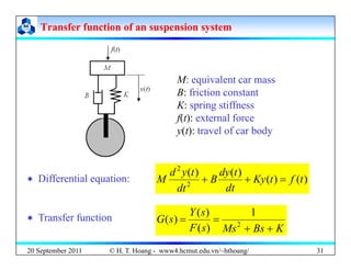
![Block diagram algebra
Block diagram algebra –
– Example 2 (cont’)
Example 2 (cont’)
‘ GB(s) = feedback loop [G2(s), H2(s)]
GC(s) = [GA(s)// unity block]
GC(s) [GA(s)// unity block]
Y(s)
Y(s)
20 September 2011 52
© H. T. Hoang - www4.hcmut.edu.vn/~hthoang/](https://image.slidesharecdn.com/introctrlsyschapter2-221125011933-bf3748c7/85/IntroCtrlSys_Chapter2-pdf-52-320.jpg)


![‘ State: The state of a system is a set of variables whose values
State of a system
State of a system
‘ State: The state of a system is a set of variables whose values,
together with the equations described the system dynamics, will
provide future state and output of the system.
A nth order system has n state variables. The state variables can be
physical variables, but not necessary.
‘ State vector: n state variables form a column vector called the
state vector.
[ ]T
n
x
x
x K
2
1
=
x
20 September 2011 72
© H. T. Hoang - www4.hcmut.edu.vn/~hthoang/](https://image.slidesharecdn.com/introctrlsyschapter2-221125011933-bf3748c7/85/IntroCtrlSys_Chapter2-pdf-72-320.jpg)
![State equations
State equations
‘ By using state variables, we can transform the n-order differential
y g ,
equation describing the system dynamics into a set of n first order
differential equations (called state equations) of the form:
⎧
⎩
⎨
⎧
=
+
=
)
(
)
(
)
(
)
(
)
(
t
t
y
t
u
t
t
Cx
B
Ax
x
&
where
⎥
⎥
⎤
⎢
⎢
⎡ n
a
a
a
a
a
a
K
K
2
22
21
1
12
11
⎥
⎥
⎤
⎢
⎢
⎡
b
b
2
1
[ ]
where
⎥
⎥
⎥
⎦
⎢
⎢
⎢
⎣
=
nn
n
n
n
a
a
a
a
a
a
K
M
M
M
K
2
1
2
22
21
A
⎥
⎥
⎥
⎦
⎢
⎢
⎢
⎣
=
n
b
b
M
2
B [ ]
n
c
c
c K
2
1
=
C
‘ Note: Depending on how we chose the state variables, a system can
be described by many different state equations.
20 September 2011 73
y y q
© H. T. Hoang - www4.hcmut.edu.vn/~hthoang/](https://image.slidesharecdn.com/introctrlsyschapter2-221125011933-bf3748c7/85/IntroCtrlSys_Chapter2-pdf-73-320.jpg)
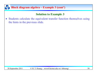
![State equations
State equations –
– Example 1
Example 1
A suspension system
A suspension system
A suspension system
A suspension system
)
(
)
(
)
(
)
(
2
t
f
t
Ky
t
dy
B
t
y
d
M =
+
+
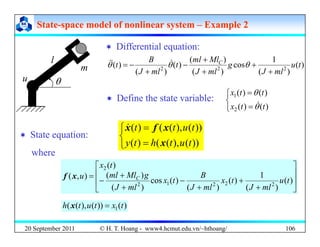
‘ Differential equation:
(*)
)
(
)
(
2
t
f
t
Ky
dt
B
dt
M =
+
+ ( )
⎪
⎨
⎧ =
1
)
(
)
( 2
1
B
K
t
x
t
x
&
‘ Denote:
⎨
⎧ = )
(
)
(
1 t
y
t
x
⎪
⎩
⎪
⎨ +
−
−
= )
(
1
)
(
)
(
)
( 2
1
2 t
f
M
t
x
M
B
t
x
M
K
t
x
&
⇒
⎩
⎨
= )
(
)
(
)
(
)
(
2
1
t
y
t
x
y
&
1
0
)
(
1
0
)
( 1
1 t
x
B
K
t
x
⎥
⎤
⎢
⎡
⎤
⎡
⎥
⎤
⎢
⎡
⎤
⎡ &
)
(
1
)
(
)
(
.
)
(
)
(
2
1
2
1
t
f
M
t
x
M
B
M
K
t
x ⎥
⎥
⎦
⎢
⎢
⎣
+
⎥
⎦
⎤
⎢
⎣
⎡
⎥
⎥
⎦
⎢
⎢
⎣
−
−
=
⎥
⎦
⎤
⎢
⎣
⎡
&
[ ] ⎤
⎡ )
(
1 t
x
⇔
[ ] ⎥
⎦
⎤
⎢
⎣
⎡
=
)
(
)
(
0
1
)
(
2
1
t
x
t
x
t
y
⎨
⎧ +
= )
(
)
(
)
( t
f
t
t B
Ax
x
&
⇔ ⎥
⎤
⎢
⎡
= B
K
1
0
A ⎥
⎤
⎢
⎡
= 1
0
B [ ]
0
1
=
C
20 September 2011 74
⎩
⎨
= )
(
)
(
)
(
)
(
)
(
t
t
y
f
Cx
⇔ ⎥
⎥
⎦
⎢
⎢
⎣
−
−
M
M
A
⎥
⎥
⎦
⎢
⎢
⎣M
B [ ]
© H. T. Hoang - www4.hcmut.edu.vn/~hthoang/](https://image.slidesharecdn.com/introctrlsyschapter2-221125011933-bf3748c7/85/IntroCtrlSys_Chapter2-pdf-74-320.jpg)


![State equations
State equations –
– Example 2 (cont’)
Example 2 (cont’)
)
(
1
)
(
)
( 1
1
t
U
L
t
x
L
K
L
R
t
x
ö
ö
ö
⎥
⎤
⎢
⎡
+
⎥
⎤
⎢
⎡
⎥
⎥
⎤
⎢
⎢
⎡ Φ
−
−
=
⎥
⎤
⎢
⎡ &
⎤
⎡ )
(
⇔
)
(
0
)
(
)
( 2
2
t
U
L
t
x
J
B
J
K
t
x
ö
ö
ö
ö
⎥
⎥
⎦
⎢
⎢
⎣
+
⎥
⎦
⎢
⎣
⎥
⎥
⎥
⎦
⎢
⎢
⎢
⎣
−
Φ
=
⎥
⎦
⎢
⎣ &
[ ] ⎥
⎦
⎤
⎢
⎣
⎡
=
)
(
)
(
1
0
)
(
2
1
t
x
t
x
t
ω
⎩
⎨
⎧
=
+
=
)
(
)
(
)
(
)
(
)
(
t
t
t
U
t
t
Cx
B
Ax
x
ω
u
&
⇔
⎤
⎡
⎥
⎥
⎥
⎤
⎢
⎢
⎢
⎡
Φ
Φ
−
−
=
B
K
L
K
L
R
ö
ö
ö
A [ ]
1
0
=
C
⎥
⎥
⎦
⎤
⎢
⎢
⎣
⎡
=
0
1
ö
L
B
where:
20 September 2011 78
⎥
⎥
⎦
⎢
⎢
⎣
−
J
J
⎥
⎦
⎢
⎣ 0
© H. T. Hoang - www4.hcmut.edu.vn/~hthoang/](https://image.slidesharecdn.com/introctrlsyschapter2-221125011933-bf3748c7/85/IntroCtrlSys_Chapter2-pdf-78-320.jpg)

![Method for establishing state equations from differential equations
Method for establishing state equations from differential equations
Case #1 (cont’)
Case #1 (cont’)
Case #1 (cont )
Case #1 (cont )
‘ State equation:
⎩
⎨
⎧
=
+
=
)
(
)
(
)
(
)
(
)
(
t
t
y
t
u
t
t
Cx
B
Ax
x
&
⎩ )
(
)
( t
t
y Cx
where:
⎤
⎡ ⎤
⎡ 0
0
1
0 ⎤
⎡ 0
⎥
⎥
⎥
⎤
⎢
⎢
⎢
⎡
)
(
)
(
)
(
2
1
t
x
t
x
M ⎥
⎥
⎥
⎤
⎢
⎢
⎢
⎡
0
1
0
0
0
0
1
0
M
M
M
M
K
K
A ⎥
⎥
⎥
⎤
⎢
⎢
⎢
⎡
0
0
M
B
⎥
⎥
⎥
⎥
⎦
⎢
⎢
⎢
⎢
⎣
=
−
)
(
)
(
)
(
1
t
x
t
x
t
n
M
x
⎥
⎥
⎥
⎥
⎥
⎢
⎢
⎢
⎢
⎢
−
−
−
−
=
−
− 1
2
1
1
0
0
0
a
a
a
a n
n
n
K
K
M
M
M
M
A
⎥
⎥
⎥
⎥
⎥
⎢
⎢
⎢
⎢
⎢
=
0
0
b
M
B
⎥
⎦
⎢
⎣ )
(t
xn ⎥
⎦
⎢
⎣ 0
0
0
0 a
a
a
a ⎥
⎦
⎢
⎣ 0
a
[ ]
0
0
0
1 K
=
C
20 September 2011 80
© H. T. Hoang - www4.hcmut.edu.vn/~hthoang/](https://image.slidesharecdn.com/introctrlsyschapter2-221125011933-bf3748c7/85/IntroCtrlSys_Chapter2-pdf-80-320.jpg)
![Method for establishing state equations from differential equations
Method for establishing state equations from differential equations
Case #1: Example
Case #1: Example
Case #1: Example
Case #1: Example
‘ Write the state equations describing the following system:
)
(
)
(
10
)
(
6
)
(
5
)
(
2 t
u
t
y
t
y
t
y
t
y =
+
+
+ &
&
&
&
&
&
⎪
⎪
⎨
⎧
=
=
)
(
)
(
)
(
)
(
1
2
1
t
x
t
x
t
y
t
x
&
‘ Define the state variables as:
⎪
⎩ = )
(
)
( 2
3 t
x
t
x &
‘ State equation:
⎩
⎨
⎧ +
=
)
(
)
(
)
(
)
(
)
( t
r
t
t
C
B
Ax
x
&
⎤
⎡
⎤
⎡
⎥
⎥
⎤
⎢
⎢
⎡
=
⎥
⎥
⎥
⎤
⎢
⎢
⎢
⎡
= 0
0
0
0
B
⎩
⎨
= )
(
)
( t
t
y Cx
where
⎥
⎥
⎥
⎦
⎤
⎢
⎢
⎢
⎣
⎡
=
⎥
⎥
⎥
⎥
⎤
⎢
⎢
⎢
⎢
⎡
=
5
2
3
5
1
0
0
0
1
0
1
0
0
0
1
0
1
2
3 a
a
a
A
⎥
⎥
⎦
⎢
⎢
⎣
=
⎥
⎥
⎥
⎦
⎢
⎢
⎢
⎣
=
5
.
0
0
0
0
0
a
b
B
20 September 2011 81
⎥
⎦
⎢
⎣ −
−
−
⎥
⎥
⎦
⎢
⎢
⎣
−
−
− 5
.
2
3
5
0
1
0
2
0
3
a
a
a [ ]
0
0
1
=
C
© H. T. Hoang - www4.hcmut.edu.vn/~hthoang/](https://image.slidesharecdn.com/introctrlsyschapter2-221125011933-bf3748c7/85/IntroCtrlSys_Chapter2-pdf-81-320.jpg)

![Method for establishing state equations from differential equations
Method for establishing state equations from differential equations
Case #2 (cont’)
Case #2 (cont’)
⎩
⎨
⎧
=
+
=
)
(
)
(
)
(
)
(
)
(
t
t
y
t
r
t
t
Cx
B
Ax
x
&
Case #2 (cont )
Case #2 (cont )
‘ State equation:
⎩ = )
(
)
( t
t
y Cx
where:
⎤
⎡ 0
0
1
0
⎥
⎥
⎥
⎤
⎢
⎢
⎢
⎡
)
(
)
(
2
1
t
x
t
x
M ⎥
⎥
⎥
⎤
⎢
⎢
⎢
⎡
0
1
0
0
0
0
1
0
M
M
M
M
K
K
⎥
⎥
⎥
⎤
⎢
⎢
⎢
⎡
β
β
2
1
⎥
⎥
⎥
⎥
⎦
⎢
⎢
⎢
⎢
⎣
=
−
)
(
)
(
)
(
1
t
t
x
t
n
M
x
⎥
⎥
⎥
⎥
⎢
⎢
⎢
⎢
−
−
−
−
=
−
− 1
2
1
1
0
0
0
a
a
a
a n
n
n
K
M
M
M
M
A
⎥
⎥
⎥
⎥
⎦
⎢
⎢
⎢
⎢
⎣
=
−
n
β
β 1
M
B
⎥
⎦
⎢
⎣ )
(t
xn ⎥
⎥
⎦
⎢
⎢
⎣ 0
0
0
0 a
a
a
a
K
[ ]
C
⎥
⎦
⎢
⎣ n
β
20 September 2011 83
[ ]
0
0
0
1 K
=
C
© H. T. Hoang - www4.hcmut.edu.vn/~hthoang/](https://image.slidesharecdn.com/introctrlsyschapter2-221125011933-bf3748c7/85/IntroCtrlSys_Chapter2-pdf-83-320.jpg)

![Method for establishing state equations from differential equations
Method for establishing state equations from differential equations
Case #2: Example
Case #2: Example
Case #2: Example
Case #2: Example
‘ Write the state equations describing the following system:
)
(
20
)
(
10
)
(
10
)
(
6
)
(
5
)
(
2 t
u
t
u
t
y
t
y
t
y
t
y +
=
+
+
+ &
&
&
&
&
&
&
‘ Define the state variables:
⎪
⎩
⎪
⎨
⎧
−
=
=
)
(
)
(
)
(
)
(
)
(
)
(
)
(
)
(
1
1
2
1
t
r
t
x
t
x
t
y
t
x
β
β
&
&
‘ The state equation:
⎩
⎨
⎧ +
=
)
(
)
(
)
(
)
(
)
( t
r
t
t
C
B
Ax
x
&
⎪
⎩ −
= )
(
)
(
)
( 2
2
3 t
r
t
x
t
x β
&
⎩
⎨
= )
(
)
( t
t
y Cx
⎤
⎡
⎤
⎡
where:
⎥
⎤
⎢
⎡ 1
β
⎥
⎥
⎥
⎦
⎤
⎢
⎢
⎢
⎣
⎡
=
⎥
⎥
⎥
⎥
⎤
⎢
⎢
⎢
⎢
⎡
=
5
2
3
5
1
0
0
0
1
0
1
0
0
0
1
0
1
2
3 a
a
a
A ⎥
⎥
⎥
⎦
⎢
⎢
⎢
⎣
=
3
2
β
β
B
20 September 2011 85
[ ]
0
0
1
=
C
⎥
⎦
⎢
⎣ −
−
−
⎥
⎥
⎦
⎢
⎢
⎣
−
−
− 5
.
2
3
5
0
1
0
2
0
3
a
a
a
© H. T. Hoang - www4.hcmut.edu.vn/~hthoang/](https://image.slidesharecdn.com/introctrlsyschapter2-221125011933-bf3748c7/85/IntroCtrlSys_Chapter2-pdf-85-320.jpg)


![State
State-
-space equations in controllable canonical form (cont’)
space equations in controllable canonical form (cont’)
‘ Write the controllable canonical state equations of the following system:
‘ Write the controllable canonical state equations of the following system:
)
(
3
)
(
)
(
4
)
(
5
)
(
)
(
2 t
u
t
u
t
y
t
y
t
y
t
y +
=
+
+
+ &
&
&
&
&
&
&
&
S l i
‘ Solution:
⎩
⎨
⎧
=
+
=
)
(
)
(
)
(
)
(
)
(
t
t
y
t
r
t
t
Cx
B
Ax
x
⎤
⎡
⎥
⎤
⎢
⎡
0
1
0
0
1
0 ⎤
⎡0
where:
⎩ )
(
)
(
y
⎥
⎥
⎥
⎦
⎤
⎢
⎢
⎢
⎣
⎡
−
−
−
=
⎥
⎥
⎥
⎥
⎥
⎦
⎢
⎢
⎢
⎢
⎢
⎣
−
−
−
=
5
.
0
5
.
2
2
1
0
0
0
1
0
1
0
0
0
1
0
1
2
3 a
a
a
A
⎥
⎥
⎥
⎦
⎤
⎢
⎢
⎢
⎣
⎡
=
1
0
0
B
⎦
⎣
⎥
⎦
⎢
⎣ 0
0
0 a
a
a
⎦
⎣
[ ]
5
.
0
0
5
.
1
0
1
2
=
⎥
⎦
⎤
⎢
⎣
⎡
=
b
b
b
C
20 September 2011 89
[ ]
0
0
0
⎥
⎦
⎢
⎣ a
a
a
© H. T. Hoang - www4.hcmut.edu.vn/~hthoang/](https://image.slidesharecdn.com/introctrlsyschapter2-221125011933-bf3748c7/85/IntroCtrlSys_Chapter2-pdf-89-320.jpg)


![Method for establishing state equations from block diagrams
Method for establishing state equations from block diagrams
Example (cont’)
Example (cont’)
Example (cont )
Example (cont )
‘ Combining (1), (2), and (3) leads to the state equations:
)
(
0
0
)
(
)
(
1
1
0
0
10
3
)
(
)
(
2
1
2
1
t
r
t
x
t
x
t
x
t
x
⎥
⎥
⎥
⎤
⎢
⎢
⎢
⎡
+
⎥
⎥
⎥
⎤
⎢
⎢
⎢
⎡
⎥
⎥
⎥
⎤
⎢
⎢
⎢
⎡
−
−
=
⎥
⎥
⎥
⎤
⎢
⎢
⎢
⎡
&
&
{
1
)
(
)
(
0
0
1
)
(
)
( 3
3
t
t
x
t
t
x
B
x
A
x
⎥
⎦
⎢
⎣
⎥
⎦
⎢
⎣
⎥
⎦
⎢
⎣−
⎥
⎦
⎢
⎣ 3
2
1
4
4 3
4
4 2
1
3
2
1
&
&
⎤
⎡ )
(t
x
‘ Output equation:
[ ]
⎥
⎥
⎥
⎦
⎤
⎢
⎢
⎢
⎣
⎡
=
=
)
(
)
(
)
(
0
0
1
)
(
)
(
3
2
1
1
t
x
t
x
t
x
t
x
t
y
4
3
4
2
1
C
20 September 2011 92
⎥
⎦
⎢
⎣ )
(
3 t
x
C
© H. T. Hoang - www4.hcmut.edu.vn/~hthoang/](https://image.slidesharecdn.com/introctrlsyschapter2-221125011933-bf3748c7/85/IntroCtrlSys_Chapter2-pdf-92-320.jpg)

![State equation to transfer function
State equation to transfer function –
– Example
Example
‘ Calculate the transfer function of the system described by the state
‘ Calculate the transfer function of the system described by the state
equation:
⎨
⎧ +
= )
(
)
(
)
( t
u
t
t B
Ax
x
&
⎩
⎨
= )
(
)
( t
t
y Cx
⎤
⎡
where
⎥
⎦
⎤
⎢
⎣
⎡
−
−
=
3
2
1
0
A ⎥
⎦
⎤
⎢
⎣
⎡
=
1
3
B [ ]
0
1
=
C
‘ Solution: The transfer function of the system is:
( ) B
A
I
C
1
)
(
)
(
)
(
−
−
=
= s
s
U
s
Y
s
G
20 September 2011 94
© H. T. Hoang - www4.hcmut.edu.vn/~hthoang/](https://image.slidesharecdn.com/introctrlsyschapter2-221125011933-bf3748c7/85/IntroCtrlSys_Chapter2-pdf-94-320.jpg)
![Calculate transfer functions from state equations
Calculate transfer functions from state equations
Example (cont’)
Example (cont’)
Example (cont )
Example (cont )
( ) ⎥
⎦
⎤
⎢
⎣
⎡
+
−
=
⎥
⎦
⎤
⎢
⎣
⎡
−
⎥
⎦
⎤
⎢
⎣
⎡
=
−
3
2
1
3
2
1
0
1
0
0
1
s
s
s
s A
I
⎦
⎣ +
⎦
⎣ −
−
⎦
⎣ 3
2
3
2
1
0 s
( ) ⎥
⎤
⎢
⎡ +
=
⎥
⎤
⎢
⎡ −
=
−
−
− s
s
s
1
3
1
1
1
1
A
I
( ) ⎥
⎦
⎢
⎣ −
−
−
+
⎥
⎦
⎢
⎣ + s
s
s
s 2
)
1
.(
2
)
3
(
3
2
( ) [ ] [ ]
1
3
1
1
3
0
1
1
1
+
=
⎥
⎤
⎢
⎡ +
=
−
−
s
s
s A
I
C( ) [ ] [ ]
1
3
2
3
2
0
1
2
3 2
2
+
+
+
=
⎥
⎦
⎢
⎣ −
+
+
= s
s
s
s
s
s
s A
I
C
( ) [ ] 1
)
3
(
3
3
1
3
1
1 +
+
=
⎥
⎤
⎢
⎡
+
=
−
− s
s
s B
A
I
C( ) [ ]
2
3
1
1
3
2
3 2
2
+
+
=
⎥
⎦
⎢
⎣
+
+
+
=
−
s
s
s
s
s
s B
A
I
C
10
3
)
(
+
s
s
G
⇒
20 September 2011 95
2
3
)
( 2
+
+
=
s
s
s
G
⇒
© H. T. Hoang - www4.hcmut.edu.vn/~hthoang/](https://image.slidesharecdn.com/introctrlsyschapter2-221125011933-bf3748c7/85/IntroCtrlSys_Chapter2-pdf-95-320.jpg)
![Solution to state equations
Solution to state equations
‘ Solution to the state equation ?
)
(
)
(
)
( t
u
t
t B
Ax
x +
=
&
∫ −
Φ
+
Φ
= +
t
d
u
t
t
t )
(
)
(
)
0
(
)
(
)
( τ
τ
τ B
x
x ∫ −
Φ
+
Φ
= d
u
t
t
t
0
)
(
)
(
)
0
(
)
(
)
( τ
τ
τ B
x
x
)]
(
[
)
( 1
s
t Φ
=
Φ −
L
where transient matrix
)]
(
[
)
( s
t Φ
=
Φ L
1
)
(
)
( −
−
=
Φ A
I
s
s
where transient matrix
‘ System response?
)
(
)
( t
t
y Cx
=
20 September 2011 96
‘ Example:
© H. T. Hoang - www4.hcmut.edu.vn/~hthoang/](https://image.slidesharecdn.com/introctrlsyschapter2-221125011933-bf3748c7/85/IntroCtrlSys_Chapter2-pdf-96-320.jpg)


![Describing nonlinear system by state equations
Describing nonlinear system by state equations
‘ A continuous nonlinear system can be described by the state
equation:
⎧ = ))
(
)
(
(
)
( t
u
t
t x
f
x
&
⎩
⎨
⎧
=
=
))
(
),
(
(
)
(
))
(
),
(
(
)
(
t
u
t
h
t
y
t
u
t
t
x
x
f
x
where: u(t): input,
y(t): output,
x(t): state vector,
x(t) = [x1(t), x2(t),…,xn(t)]T
f(.), h(.): nonlinear functions
20 September 2011 104
© H. T. Hoang - www4.hcmut.edu.vn/~hthoang/](https://image.slidesharecdn.com/introctrlsyschapter2-221125011933-bf3748c7/85/IntroCtrlSys_Chapter2-pdf-104-320.jpg)


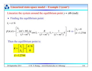


![Linearized state
Linearized state-
-space model
space model –
– Example 2 (cont’)
Example 2 (cont’)
‘ The output matrix around the equilibrium point:
‘ The output matrix around the equilibrium point:
1
1
1 =
∂
∂
=
x
h
c
[ ]
2
1 c
c
=
C 0
)
(
2
2 =
∂
∂
=
x
h
c
)
(
1
∂ u
x ,
x )
(
2 u
,
x
1
d
=
D 0
)
(
1 =
∂
∂
=
u
h
d
)
(
∂ u
u ,
x
‘ Then the linearized state equation is:
⎩
⎨
⎧ +
=
)
(
~
)
(
~
)
(
~
)
(
~
)
(
~
)
(
~
t
t
t
t
u
t
t
D
C
B
x
A
x
&
⎩ +
= )
(
)
(
)
( t
u
t
t
y D
x
C
⎥
⎤
⎢
⎡
=
1
0
A ⎥
⎤
⎢
⎡
=
0
B [ ]
0
1
=
C 0
=
D
⎥
⎦
⎢
⎣
=
22
21 a
a
A ⎥
⎦
⎢
⎣
=
2
b
B [ ]
0
1
C 0
=
D
20 September 2011 119
)
(
)
,
( 1 t
x
u
h =
x
© H. T. Hoang - www4.hcmut.edu.vn/~hthoang/](https://image.slidesharecdn.com/introctrlsyschapter2-221125011933-bf3748c7/85/IntroCtrlSys_Chapter2-pdf-119-320.jpg)


![Attack surfaces and attack tress[inform]](https://cdn.slidesharecdn.com/ss_thumbnails/lecture03-260108015941-a4dee53b-thumbnail.jpg?width=640&height=640&fit=bounds)


