SlideShare a Scribd company logo
Mathematics for Economists
Chapters 4-5
Linear Models and Matrix Algebra
Johann Carl Friedrich Gauss (1777–1855)
The Nine Chapters on the Mathematical Art
(1000-200 BC)
Objectives of math for economists
 To understand mathematical economics problems by stating
the unknown, the data and the conditions
 To plan solutions to these problems by finding a connection
between the data and the unknown
 To carry out your plans for solving mathematical economics
problems
 To examine the solutions to mathematical economics
problems for general insights into current and future
problems
 Remember: Math econ is like love – a simple idea but it can
get complicated.
2
4. Linear Algebra
 Some history:
 The beginnings of matrices and determinants goes back to
the second century BC although traces can be seen back to
the fourth century BC. But, the ideas did not make it to
mainstream math until the late 16th
century
 The Babylonians around 300 BC studied problems which
lead to simultaneous linear equations.
 The Chinese, between 200 BC and 100 BC, came much closer
to matrices than the Babylonians. Indeed, the text Nine
Chapters on the Mathematical Art written during the Han
Dynasty gives the first known example of matrix methods.
 In Europe, two-by-two determinants were considered by
Cardano at the end of the 16th
century and larger ones by
Leibniz and, in Japan, by Seki about 100 years later.
4. What is a Matrix?
 A matrix is a set of elements, organized into rows and columns






dc
ba
rows
columns
• a and d are the diagonal elements.
• b and c are the off-diagonal elements.
• Matrices are like plain numbers in many ways: they can be added,
subtracted, and, in some cases, multiplied and inverted (divided).
4. Matrix: Details
 Examples:
5
[ ]δβα=





−
= b
d
b
A ;
1
1
• Dimensions of a matrix: numbers of rows by numbers of
columns. The Matrix A is a 2x2 matrix, b is a 1x3 matrix.
• A matrix with only one column or only one row is called a
vector.
• If a matrix has an equal numbers of rows and columns, it is
called a square matrix. Matrix A, above, is a square matrix.
• Usual Notation: Upper case letters => matrices
Lower case => vectors
4.1 Basic Operations
Addition, Subtraction, Multiplication






++
++
=





+





hdgc
fbea
hg
fe
dc
ba






−−
−−
=





−





hdgc
fbea
hg
fe
dc
ba






++
++
=











dhcfdgce
bhafbgae
hg
fe
dc
ba
Just add elements
Just subtract elements
Multiply each row
by each column






=





kdkc
kbka
dc
ba
k Multiply each
element by the scalar
4.1 Matrix multiplication: Details
 Multiplication of matrices requires a conformability condition
 The conformability condition for multiplication is that the
column dimensions of the lead matrix A must be equal to the
row dimension of the lag matrix B.
 What are the dimensions of the vector, matrix, and result?
[ ] [ ]131211
232221
131211
1211 cccc
bb
bbb
aaaB ==








=
7
[ ]231213112212121121121111 babababababa +++=
• Dimensions: a(1x2), B(2x3) => c(1x3)
4.1 Basic Matrix Operations: Examples
222222
117
25
20
13
97
12
xxx CBA =+






=





+





Matrix addition
Matrix subtraction
Matrix multiplication
Scalar multiplication
8






=





−





65
11
32
01
97
12
222222 x
2726
34
32
01
x
97
12
xxx CBA =






=

















=





8143
2141
16
42
8
1
4.1 Laws of Matrix Addition & Multiplication






++
++
=





+





=+
22222121
12121111
2221
1211
2221
1211
abaa
abba
bb
bb
aa
aa
BA
 Commutative law of Matrix Addition: A + B = B + A
9






++
++
=





+





=+
22222121
12121111
2221
1211
2221
1211
abab
abab
bb
aa
bb
bb
AB
 Matrix Multiplication is distributive across Additions:
A (B+ C) = AB + AC (assuming comformability applies).
4.1 Matrix Multiplication
 Matrix multiplication is generally not commutative. That is,
AB ≠ BA even if BA is conformable
(because diff. dot product of rows or col. of A&B)





 −
=





=
76
10
,
43
21
BA
10
( ) ( ) ( ) ( )
( ) ( ) ( ) ( ) 





=





+−+
+−+
=
2524
1312
74136403
72116201
AB
( ) ( )( ) ( ) ( )
( ) ( ) ( ) ( ) 




 −−
=





++
−+−+
=
4027
43
47263716
41203110
BA
4.1 Matrix multiplication
 Exceptions to non-commutative law:
AB=BA iff
B = a scalar,
B = identity matrix I, or
B = the inverse of A -i.e., A-1
11
 Theorem: It is not true that AB = AC => B=C
Proof:










−−−=









 −
=










−−
−=
132
111
212
;
011
010
111
;
321
101
121
CBA
Note: If AB = AC for all matrices A, then B=C.
4.1 Transpose Matrix










−
=′=>




 −
=
49
08
13
401
983
AA:Example
 The transpose of a matrix A is another matrix AT
(also written A
′) created by any one of the following equivalent actions:
- write the rows (columns) of A as the columns (rows) of AT
- reflect A by its main diagonal to obtain AT
 Formally, the (i,j) element of AT
is the (j,i) element of A:
[AT
]ij
= [A]jj
 If A is a m × n matrix => AT
is a n × m matrix.
 (A')' = A
 Conformability changes unless the matrix is square.
12
4.1 Inverse of a Matrix
 Identity matrix:
AI = A










=
100
010
001
I
Notation: Ij is a jxj identity matrix.
 Given A (mxn), the matrix B (nxm) is a right-inverse for A iff
AB = Im
 Given A (mxn), the matrix C (mxn) is a left-inverse for A iff
CA = In
4.1 Inverse of a Matrix
 Inversion is tricky:
(ABC)-1
= C-1
B-1
A-1
 More on this topic later
 Theorem: If A (mxm), has both a right-inverse B and a left-inverse C,
thenC = B.
Proof:
AB=Im and CA=In. Thus,
C(AB)=C Im = C and C(AB)=(CA)B=InB=B
=> C(nxm)=B(mxn)
Note:
- This matrix is unique.
- If A has both a right and a left inverse, it is called invertible.
4.1 Vector multiplication: Geometric
interpretation
 Think of a vector as a
directed line segment in N-
dimensions! (has “length”
and “direction”)
 Scalar multiplication
(“scales” the vector –i.e.,
changes length)
 Source of linear
dependence
15
[ ]6 4 2= U
[ ]3 2 = U
[ ]− ⋅ = − −1 3 2U
x2
x1
-4 -3 -2 -1 1 2 3 4 5 6
6
5
4
3
2
1
-2
4.1 Vector Addition: Geometric
interpretation
 v' = [2 3]
 u' = [3 2]
 w’= v'+u' = [5 5]
 Note that two vectors
plus the concepts of
addition and
multiplication can create
a two-dimensional space.
16
x1
x2
5
4
3
2
1
1 2 3 4 5
w
u
v
u
A vector space is a mathematical structure formed by a collection of
vectors, which may be added together and multiplied by scalars. (It’s
closed under multiplication and addition).
4.1 Vector Space
 Given a field R and a set V of objects, on which “vector
addition” (VxV→V), denoted by “+”, and “scalar
multiplication” (RxS →V), denoted by “. ”, are defined.
If the following axioms are true for all objects u, v, and w in V
and all scalars c and k in R, then V is called a vector space and the
objects in V are called vectors.
1. u+v  is in V (closed under addition).
2. u + v = v + u (vector addition is commutative).
3. θ is in V, such that u+ θ = u (null element).
4. u + (v+w) = (v + u) +w (distributive law of vector addition)
5. For each v, there is a –v, such that v+(-v) = θ
6. c .u is in V (closed under scalar multiplication).
7. c. (k . u) = (c .k) u (scalar multiplication is associative).17
4.1 Vector Space
8. c. (v+ u) = (c. v)+ (c. u)
9. (c+k) . u = (c. u)+ (k. u)
10. 1.u=u (unit element).
11. 0.u= θ (zero element).
We can write S = {V,R,+,.}to denote an abstract vector space.
This is a general definition. If the field R represents the real
numbers, then we define a real vector space.
 Definition: Linear Combination
Given vectors u1,...,uk,, the vector w = c1 u1+....+ ckuk is called a linear
combination of the vectors u ,...,u .
18
4.1 Vector Space
 Definition: Subspace
Given the vector space V and W a sect of vectors, such that W is
in V. Then W is a subspace iff:
u, v are in W => u+v are in W, and
c u is in W for every c in R.
u1,...,uk,, the vector w = c1 u1+....+ ckuk is called a linear combination of
the vectors u1,...,uk,.
19
4.1 System of equations: Matrices and4.1 System of equations: Matrices and
VectorsVectors
Assume an economic model as system of linear
equations in which
aij parameters, where i = 1.. n rows, j = 1.. m columns,
and n=m
xi endogenous variables,
di exogenous variables and constants
nn
n
n
nm
m
m
nn d
d
d
x
x
x
ax
ax
ax
axa
axa
axa






2
1
2
22
12
211
22121
12111
=
=
=
+
+
+
+
+
+
20
 A general form matrix of a system of linear equations
Ax = d where
A = matrix of parameters
x = column vector of endogenous variables
d = column vector of exogenous variables and constants
 Solve for x*
dAx
dAx
d
d
d
x
x
x
aaa
aaa
aaa
nnnmnn
m
m
1*
2
1
2
1
21
22221
11211
−
=
=












=





























21
4.1 System of equations: Matrices and4.1 System of equations: Matrices and
VectorsVectors
4.1 Solution of a General-equation System
 Assume the 2x2 model
2x + y = 12
4x + 2y = 24
Find x*, y*:
y = 12 – 2x
4x + 2(12 – 2x) = 24
4x +24 – 4x = 24
0 = 0 ? indeterminante!
 Why?
4x + 2y =24
2(2x + y) = 2(12)
 one equation with two
unknowns
2x + y = 12
x, y
Conclusion:
not all simultaneous equation
models have solutions
(not all matrices have inverses).
22
4.1 Linear dependence
 A set of vectors is linearly dependent if any one of them can
be expressed as a linear combination of the remaining
vectors; otherwise, it is linearly independent.
 Formal definition: Linear independent
The set {u1,...,uk} is called a linearly independent set of vectors
iff
c1 u1+....+ ckuk = θ => c1= c2=...=ck,=0.
 Notes:
- Dependence prevents solving a system of equations. More
unknowns than independent equations.
- The number of linearly independent rows or columns in a
matrix is the rank of a matrix (rank(A)). 23
4.1 Linear dependence
 Examples: [ ]
[ ]
//
2
/
1
'
2
'
1
'
2
'
1
02
2412
105
2410
125
=−








=





=
=
vv
v
v
v
v
24
[ ] [ ]
[ ]
023
54
162216
23
5
4
;
8
1
;
7
2
321
3
21
321
=−−
==
−=
−






=





=





=
vvv
v
vv
vvv
4.2 Application 1: One Commodity Market
Model (2x2 matrix)
Economic Model
1) Qd = a – bP (a,b >0)
2) Qs = -c + dP (c,d >0)
3) Qd= Qs
 Find P* and Q*
Scalar Algebra form
(Endogenous Vars :: Constants)
4) 1Q + bP = a
5) 1Q – dP = -c
25
db
bcad
Q
db
ca
P
+
−
=
+
+
=
*
*
4.2 One Commodity Market Model
(2x2 matrix)
26
dAx
c
a
d
b
P
Q
dAx
c
a
P
Q
d
b
1*
1
*
*
1
1
1
1
−
−
=






−





−
=





=






−
=











−
Matrix algebra
4.2 Application II: Three Equation4.2 Application II: Three Equation
National Income Model (3x3 matrix)National Income Model (3x3 matrix)
 Model
Y = C + I0
+ G0
C = a + b (Y-T) (a > 0, 0<b<1)
T = d + t Y (d > 0, 0<t<1)
 Endogenous variables?
 Exogenous variables?
 Constants?
 Parameters?
 Why restrictions on the parameters?
27
4.2 Three Equation National Income4.2 Three Equation National Income
ModelModel Endogenous: Y, C, T: Income (GNP), Consumption, and
Taxes.
 Exogenous: I0 and G0: autonomous Investment & Government
spending.
 Parameters:
a & d: autonomous consumption and taxes.
t: marginal propensity to tax gross income 0 < t < 1.
b: marginal propensity to consume private goods and services
from gross income 0 < b < 1.
 Solution:
28
btb
GIbda
Y
+−
++−
=
1
00*
4.2 Three Equation National Income Model
Parameters &
Endogenous vars.
Exog.
vars.
Y C T &cons.
1Y -1C +0T = I0+G0
-bY +1C +bT = a
-tY +0C +1T = d
 Given (Model)
Y = C + I0
+ G0
C = a + b (Y-T)
T = d + t Y
 Find Y*, C*, T*
29









 +
=




















−
−
−
d
a
GI
T
C
Y
t
bb
00
10
1
011
dAx
dAx
1* −
=
=
4.2 Three Equation National Income Model
30
dAx
d
a
GI
t
bb
T
C
Y
dAx
d
a
GI
T
C
Y
t
bb
1*
00
1
*
*
*
00
10
1
011
10
1
011
−
−
=









 +










−
−
−
=










=









 +
=




















−
−
−
4.3 Notes on Vector Operations






=
2
3
12x
u
An [m x 1] column vector u and a
[1 x n] row vector v, yield a
product matrix uv of dimension
[m x n].
31
[ ]541
31
=′
x
v
[ ] 





=





=′
10
15
8
12
2
3
541
2
3
32x
vu
4.3 Vector multiplication: Dot (inner),
and cross product
• The dot product produces a scalar! c’z =1x1=1x4 4x1= z’c
32
44332211 zczczczcy +++=
∑=
=
4
1i
ii zcy
[ ] zc'
4
3
2
1
4321 =












=
z
z
z
z
ccccy
4.3 Vectors: Dot Product
[ ] cfbead
f
e
d
cbaT
++=










==⋅ αββα
ccbbaaT
++== 2/1
][ααα
)cos(θβαβα =⋅
Think of the dot product
as a matrix multiplication
The magnitude (length) is the
square root of the dot
product of a vector with
itself.
The dot product is also related
to the angle between the two
vectors – but it doesn’t tell us
the angle.
Note: As the cos(90) is zero, the dot product of two orthogonal vectors is zero.
4.3 Vectors: Magnitude and Phase (direction)
x
y
||v||
θ
Alternate representations:
Polar coords: (||v||, θ)
Complex numbers: ||v||ejθ
“phase”
runit vectoais,1If
1
2
),,
2
,
1
(
vv
n
i
i
xv
n
xxxv
=
=
=
=
∑
 T
(Magnitude or “2-norm”)
(unit vector => pure direction)
4.3 Vectors: Cross Product
 The cross product of vectors A and B is a vector C which
is perpendicular to A and B
 The magnitude of C is proportional to the cosine of the
angle between A and B
 The direction of C follows the right hand rule – this why we
call it a “right-handed coordinate system”
)sin(θbaba =×
4.3 Vectors: Cross Product: Right hand rule
4.3 Vectors: Norm
• Given a vector space V, the function g: V→ R is called a norm
if and only if:
1) g(x)≥ 0, for all xεV
2) g(x)=0 iff x=θ (empty set)
3) g(αx) = |α|g(x) for all αεR, xεV
4) g(x+y)=g(x)+g(y) (“triangle inequality”) for all x,yεV
The norm is a generalization of the notion of size or length of a
vector.
• An infinite number of functions can be shown to qualify as
norms. For vectors in Rn
, we have the following examples:
g(x)=maxi (xi), g(x)=∑i |xi|, g(x)=[∑i (xi)4
] ¼
• Given a norm on a vector space, we can define a measure of
“how far apart” two vectors are using the concept of a metric.
4.3 Vectors: Metric
• Given a vector space V, the function d: VxV→ R is called a
metric if and only if:
1) d(x,y)≥ 0, for all x,yεV
2) d(x,y)=0 iff x=y
3) d(x,y) = d(y,x) for all x,yεV
4) d(x+y)≤d(x,z) + d(z,y) (“triangle inequality”) for all x,y,zεV
Given a norm g(.), we can define a metric by the equation:
d(x,y) = g(x-y).
• The dot product is called the Euclidian distance metric.
4.3 Orthonormal Basis
 Basis: a space is totally defined by a set of vectors – any point is
a linear combination of the basis
 Ortho-Normal: orthogonal + normal
 Orthogonal: dot product is zero
 Normal: magnitude is one
 Example: X, Y, Z (but don’t have to be!)
[ ]
[ ]
[ ]T
T
T
z
y
x
100
010
001
=
=
=
0
0
0
=⋅
=⋅
=⋅
zy
zx
yx
• X, Y, Z is an orthonormal basis. We can describe any 3D point
as a linear combination of these vectors.
4.3 Orthonormal Basis










⋅+⋅+⋅
⋅+⋅+⋅
⋅+⋅+⋅
=




















ncnbna
vcvbva
ucubua
nvu
nvu
nvu
c
b
a
333
222
111
00
00
00
(not an actual formula – just a way of thinking about it)
• To change a point from one coordinate system to another,
compute the dot product of each coordinate row with each of
the basis vectors.
• How do we express any point as a combination of a new basis U,
V, N, given X, Y, Z?
4.5 Identity and Null Matrices


























000
000
000
.
100
010
001
10
01
etc
or Identity Matrix is a square matrix and also
it is a diagonal matrix with 1 along the
diagonals. Similar to scalar “1”
 Null matrix is one in which all elements
are zero. Similar to scalar “0”
 Both are diagonal matrices
 Both are idempotent matrices:
A = AT
and
A = A2
= A3
= … 41
4.6 Inverse matrix
 AA-1
= I
 A-1
A=I
 Necessary for matrix to be
square to have unique inverse
 If an inverse exists for a
square matrix, it is unique
 (A')-1
=(A-1
)'
42
• A x = d
• A-1
A x = A-1
d
• Ix = A-1
d
• x = A-1
d
• Solution depends on A-1
• Linear independence
• Determinant test!
4.6 Inverse of a Matrix










100
010
001
|
ihg
fed
cba
1. Append the identity matrix to
A
2. Subtract multiples of the
other rows from the first row
to reduce the diagonal
element to 1
3. Transform the identity matrix
as you go
4. When the original matrix is
the identity, the identity has
become the inverse!
4.6 Determination of the Inverse
(Gauss-Jordan Elimination)
AX = I
I X = K
I X = X = A-1
K = A-1
1) Augmented
matrix
all A, X and I are (nxn)
square matrices
X = A-1
Gauss elimination Gauss-Jordan
eliminationU: upper triangular
further row
operations
[A I ] [ U H] [ I K]
2) Transform
augmented matrix
4.6 Determinant of a Matrix
 The determinant is a number associated with any squared
matrix.
 If A is an nxn matrix, the determinant is given by |A| or
det(A).
 Determinants are used to characterize invertible matrices. A
matrix is invertible (non-singular) if and only if it has a non-
zero determinant
 That is, if |A|≠0 → A is invertible.
 Determinants are used to describe the solution to a system of
linear equations with Cramer's rule.
 Can be found using factorials, pivots, and cofactors! More on
this later.
 Lots of interpretations 45
4.6 Determinant of a Matrix
 Used for inversion. Example: Inverse of a 2x2 matrix:






=
dc
ba
A bcadAA −== )det(||






−
−
−
=−
ac
bd
bcad
A
11
This matrix is called the
adjugate of A (or adj(A)).
A-1
= adj(A)/|A|
4.6 Determinant of a Matrix (3x3)
cegbdiafhcdhbfgaei
ihg
fed
cba
−−−++=
ihg
fed
cba
ihg
fed
cba
ihg
fed
cba
Sarrus’ Rule: Sum
from left to right.
Then, subtract from
right to left
Note: N! terms
4.6 Determinants: Laplace formula
 The determinant of a matrix of arbitrary size can be defined
by the Leibniz formula or the Laplace formula.
 The Laplace formula (or expansion) expresses the determinant |
A| as a sum of n determinants of (n-1) × (n-1) sub-matrices
of A. There are n2
such expressions, one for each row and
column of A
 Define the i,j minor Mij (usually written as |Mij|) of A as the
determinant of the (n-1) × (n-1) matrix that results from
deleting the i-th row and the j-th column of A.
48
Pierre-Simon Laplace (1749–1827).
4.6 Determinants: Laplace formula
 Define the Ci,jthe cofactor of A as:
49
||)1( ,, ji
ji
ji MC +
−=
• The cofactor matrix of A -denoted by C-, is defined as the nxn
matrix whose (i,j) entry is the (i,j) cofactor of A. The transpose
of C is called the adjugate or adjoint of A (adj(A)).
• Theorem (Determinant as a Laplace expansion)
Suppose A = [aij] is an nxn matrix and i,j= {1, 2, ...,n}. Then
the determinant
njnjjjijij
ininiiii
CaCaCa
CaCaCaA
+++=
+++=
...
...||
22
2211
4.6 Determinants: Laplace formula
 Example:
50










−=
642
010
321
A
0)0(x4)3x2-x61)(1()0(x2
0))2x)1((x3)0(x)1(x2)6x1(x1
x3x2x1|| 131211
=−+−+−=
=−−+−+−=
=++= CCCA
 |A| is zero => The matrix is non-singular. (Check!)
4.6 Determinants: Properties
 Interchange of rows and columns does not affect |A|.
(Corollary, |A| = |A’|.)
 |kA| = kn
|A|, where k is a scalar.
 |I| = 1, where I is the identity matrix.
 |A| = |A’|.
 |AB| = |A||B|.
 |A-1
|=1/|A|.
51
4.6 Matrix inversion: Note
 It is not possible to divide one matrix by another. That is, we
can not write A/B. For two matrices A and B, the quotient can
be written as AB-1
or B-1
A.
 In general, in matrix algebra AB-1
≠ B-1
A.
Thus, writing A/B does not clearly identify whether it represents
AB-1
or B-1
A.
We’ll say B-1
post-multiplies A (for AB-1
) and
B-1
pre-multiplies A (for B-1
A)
 Matrix division is matrix inversion.
52
4.7 Application IV: Finite Markov Chains
Markov processes are used to measure
movements over time.
53
[ ] [ ]
[ ] [ ] [ ]
[ ] [ ]
[ ]90110
100*6.100*3.,100*4.100*7.
6.4.
3.7.
100100
PP
PP
x
plant?eachatbewillemployeesmanyhowyear,oneofendAt the
6.4.
3.7.
PP
PP
M
yprobabilitknownaw/plantseachbetweenmoveandstayemployeesThe
100100x
B&Aplantsover twoddistributeare0at timeEmployees
0000
BBBA
ABAA
00
/
011
BBBA
ABAA
00
/
0
=
++=





=
++=





==






=





=
==
BBABBAAA PBPBPAPABAMBA
BA
4.7 Application IV: Finite Markov Chains
 Associative law of multiplication
54
[ ] [ ] [ ]
[ ] [ ]
[ ] [ ] [ ]8711390*6.110*3.90*4.110*7.
6.4.
3.7.
90110
PP
PP
PP
PP
x
90110
PP
PP
x
plant?eachatbewillemployeesmanyhowyears,twoofendAt the
BBBA
ABAA
BBBA
ABAA
00
2/
022
BBBA
ABAA
00
/
011
=++=





=












==
=





==
BAMBA
BAMBA
Ch. 4 Linear Models & Matrix Algebra:
Summary
 Matrix algebra can be used:
a. to express the system of
equations in a compact notation;
b. to find out whether solution to a
system of equations exist; and
c. to obtain the solution if it exists.
Need to invert the A matrix to
find the solution for x*
55
d
A
adjA
x
A
adjA
A
dAx
dAx
=
=
=
=
−
−
*
1
1*
det
Ch. 4 Notation and Definitions: Summary
 A (Upper case letters) = matrix
 b (Lower case letters) = vector
 nxm = n rows, m columns
 rank(A) = number of linearly independent vectors of A
 trace(A) = tr(A) = sum of diagonal elements of A
 Null matrix = all elements equal to zero.
 Diagonal matrix = all non-zero elements are in the
diagonal.
 I = identity matrix (diagonal elements: 1, off-diagonal:0)
 |A| = det(A) = determinant of A
 A-1
= inverse of A
 A’=AT
= Transpose of A
 A=AT
Symmetric matrix
 A=A-1
Orthogonal matrix
|Mij|= Minor of A
56
You know too much linear algebra when...
You look at the long row of milk cartons at Whole
Foods --soy, skim, .5% low-fat, 1% low-fat, 2% low-fat,
and whole-- and think: "Why so many? Aren't soy, skim,
and whole a basis?"

More Related Content

What's hot

Mathematics for economics
Mathematics for economicsMathematics for economics
Mathematics for economics
8891743524
 
Introduction to Econometrics
Introduction to EconometricsIntroduction to Econometrics
Introduction to Econometrics
Almaszabeen Badekhan
 
Keynesian model with multiplier
Keynesian model with multiplierKeynesian model with multiplier
Keynesian model with multiplier
Michael Noel
 
Theories of the Consumption Function 1
Theories of the Consumption Function 1Theories of the Consumption Function 1
Theories of the Consumption Function 1
Prabha Panth
 
Heteroscedasticity Remedial Measures.pptx
Heteroscedasticity Remedial Measures.pptxHeteroscedasticity Remedial Measures.pptx
Heteroscedasticity Remedial Measures.pptx
PatilDevendra5
 
Introduction to Econometrics
Introduction to EconometricsIntroduction to Econometrics
Introduction to Econometrics
RajendranC4
 
Econometrics ch2
Econometrics ch2Econometrics ch2
Econometrics ch2
Baterdene Batchuluun
 
Elasticity of substitution
Elasticity of substitutionElasticity of substitution
Elasticity of substitution
Pabitra Mishra
 
The Economic Problem. Scarcity and Choice
The Economic Problem. Scarcity and ChoiceThe Economic Problem. Scarcity and Choice
The Economic Problem. Scarcity and Choice
Shanique Elliott
 
Econometrics
EconometricsEconometrics
Econometrics
Pawan Kawan
 
MModule 1 ppt.pptx
MModule 1 ppt.pptxMModule 1 ppt.pptx
MModule 1 ppt.pptx
jyotikumarijyotshna
 
Gregory mankiw macroeconomic 7th edition chapter (17)
Gregory mankiw macroeconomic 7th edition chapter  (17)Gregory mankiw macroeconomic 7th edition chapter  (17)
Gregory mankiw macroeconomic 7th edition chapter (17)
Kyaw Thiha
 
Econometrics ch1
Econometrics ch1Econometrics ch1
Econometrics ch1
Baterdene Batchuluun
 
Multiplier-Accelerator Interaction
Multiplier-Accelerator InteractionMultiplier-Accelerator Interaction
Multiplier-Accelerator Interaction
manuelmathew1
 
Dummy variables
Dummy variablesDummy variables
Dummy variables
Irfan Hussain
 
Gregory mankiw macroeconomic 7th edition chapter (15)
Gregory mankiw macroeconomic 7th edition chapter  (15)Gregory mankiw macroeconomic 7th edition chapter  (15)
Gregory mankiw macroeconomic 7th edition chapter (15)
Kyaw Thiha
 
Eco Basic 1 8
Eco Basic 1 8Eco Basic 1 8
Eco Basic 1 8
kit11229
 
Ch. 2-optimization-techniques
Ch. 2-optimization-techniquesCh. 2-optimization-techniques
Ch. 2-optimization-techniques
anj134u
 
Mankiw6e chap11
Mankiw6e chap11Mankiw6e chap11
Linear programing
Linear programingLinear programing
Linear programing
anam katmale
 

What's hot (20)

Mathematics for economics
Mathematics for economicsMathematics for economics
Mathematics for economics
 
Introduction to Econometrics
Introduction to EconometricsIntroduction to Econometrics
Introduction to Econometrics
 
Keynesian model with multiplier
Keynesian model with multiplierKeynesian model with multiplier
Keynesian model with multiplier
 
Theories of the Consumption Function 1
Theories of the Consumption Function 1Theories of the Consumption Function 1
Theories of the Consumption Function 1
 
Heteroscedasticity Remedial Measures.pptx
Heteroscedasticity Remedial Measures.pptxHeteroscedasticity Remedial Measures.pptx
Heteroscedasticity Remedial Measures.pptx
 
Introduction to Econometrics
Introduction to EconometricsIntroduction to Econometrics
Introduction to Econometrics
 
Econometrics ch2
Econometrics ch2Econometrics ch2
Econometrics ch2
 
Elasticity of substitution
Elasticity of substitutionElasticity of substitution
Elasticity of substitution
 
The Economic Problem. Scarcity and Choice
The Economic Problem. Scarcity and ChoiceThe Economic Problem. Scarcity and Choice
The Economic Problem. Scarcity and Choice
 
Econometrics
EconometricsEconometrics
Econometrics
 
MModule 1 ppt.pptx
MModule 1 ppt.pptxMModule 1 ppt.pptx
MModule 1 ppt.pptx
 
Gregory mankiw macroeconomic 7th edition chapter (17)
Gregory mankiw macroeconomic 7th edition chapter  (17)Gregory mankiw macroeconomic 7th edition chapter  (17)
Gregory mankiw macroeconomic 7th edition chapter (17)
 
Econometrics ch1
Econometrics ch1Econometrics ch1
Econometrics ch1
 
Multiplier-Accelerator Interaction
Multiplier-Accelerator InteractionMultiplier-Accelerator Interaction
Multiplier-Accelerator Interaction
 
Dummy variables
Dummy variablesDummy variables
Dummy variables
 
Gregory mankiw macroeconomic 7th edition chapter (15)
Gregory mankiw macroeconomic 7th edition chapter  (15)Gregory mankiw macroeconomic 7th edition chapter  (15)
Gregory mankiw macroeconomic 7th edition chapter (15)
 
Eco Basic 1 8
Eco Basic 1 8Eco Basic 1 8
Eco Basic 1 8
 
Ch. 2-optimization-techniques
Ch. 2-optimization-techniquesCh. 2-optimization-techniques
Ch. 2-optimization-techniques
 
Mankiw6e chap11
Mankiw6e chap11Mankiw6e chap11
Mankiw6e chap11
 
Linear programing
Linear programingLinear programing
Linear programing
 

Viewers also liked

Mercurial setup
Mercurial setupMercurial setup
Mercurial setup
Melvin Cabatuan
 
Tecnología y guerra
Tecnología y guerraTecnología y guerra
Tecnología y guerra
jose polania
 
STS-Sanita
STS-SanitaSTS-Sanita
STS-Sanita
Paolo Giorgini
 
1555 linear equations
1555 linear equations1555 linear equations
1555 linear equations
Dr Fereidoun Dejahang
 
Presentación1
Presentación1Presentación1
Presentación1inquietos
 
Recruitment and selection
Recruitment and selectionRecruitment and selection
Recruitment and selection
mayank6802
 
Реализация международных инфраструктурных проектов
Реализация международных инфраструктурных проектов Реализация международных инфраструктурных проектов
Реализация международных инфраструктурных проектов
Unison Group
 
1579 parametric equations
1579 parametric equations1579 parametric equations
1579 parametric equations
Dr Fereidoun Dejahang
 
Dissertation_FilipaOliveiraMartins
Dissertation_FilipaOliveiraMartinsDissertation_FilipaOliveiraMartins
Dissertation_FilipaOliveiraMartins
Filipa Oliveira Martins
 
Letter of Congratulations - C&Q Level 1
Letter of Congratulations - C&Q Level 1Letter of Congratulations - C&Q Level 1
Letter of Congratulations - C&Q Level 1
Mohamed Nabih El Shimi
 
ircpvpcfinalen
ircpvpcfinalenircpvpcfinalen
ircpvpcfinalen
Sonia Rastogi, MPH
 
Amal arb1.0 v3
Amal arb1.0 v3Amal arb1.0 v3
Amal arb1.0 v3
zishank
 
11.teach yourself arabic (1986)
11.teach yourself arabic (1986)11.teach yourself arabic (1986)
11.teach yourself arabic (1986)
Mohammad Ali
 
04.arabic writing for beginners
04.arabic writing for beginners04.arabic writing for beginners
04.arabic writing for beginners
Mohammad Ali
 

Viewers also liked (14)

Mercurial setup
Mercurial setupMercurial setup
Mercurial setup
 
Tecnología y guerra
Tecnología y guerraTecnología y guerra
Tecnología y guerra
 
STS-Sanita
STS-SanitaSTS-Sanita
STS-Sanita
 
1555 linear equations
1555 linear equations1555 linear equations
1555 linear equations
 
Presentación1
Presentación1Presentación1
Presentación1
 
Recruitment and selection
Recruitment and selectionRecruitment and selection
Recruitment and selection
 
Реализация международных инфраструктурных проектов
Реализация международных инфраструктурных проектов Реализация международных инфраструктурных проектов
Реализация международных инфраструктурных проектов
 
1579 parametric equations
1579 parametric equations1579 parametric equations
1579 parametric equations
 
Dissertation_FilipaOliveiraMartins
Dissertation_FilipaOliveiraMartinsDissertation_FilipaOliveiraMartins
Dissertation_FilipaOliveiraMartins
 
Letter of Congratulations - C&Q Level 1
Letter of Congratulations - C&Q Level 1Letter of Congratulations - C&Q Level 1
Letter of Congratulations - C&Q Level 1
 
ircpvpcfinalen
ircpvpcfinalenircpvpcfinalen
ircpvpcfinalen
 
Amal arb1.0 v3
Amal arb1.0 v3Amal arb1.0 v3
Amal arb1.0 v3
 
11.teach yourself arabic (1986)
11.teach yourself arabic (1986)11.teach yourself arabic (1986)
11.teach yourself arabic (1986)
 
04.arabic writing for beginners
04.arabic writing for beginners04.arabic writing for beginners
04.arabic writing for beginners
 

Similar to 1560 mathematics for economists

Linear Algebra and Matrix
Linear Algebra and MatrixLinear Algebra and Matrix
Linear Algebra and Matrix
itutor
 
Bba i-bm-u-2- matrix -
Bba i-bm-u-2- matrix -Bba i-bm-u-2- matrix -
Bba i-bm-u-2- matrix -
Rai University
 
matrix-algebra-for-engineers (1).pdf
matrix-algebra-for-engineers (1).pdfmatrix-algebra-for-engineers (1).pdf
matrix-algebra-for-engineers (1).pdf
ShafaqMehmood2
 
Linear Algebra Assignment help
Linear Algebra Assignment helpLinear Algebra Assignment help
Linear Algebra Assignment help
Maths Assignment Help
 
Introduction To Matrix
Introduction To MatrixIntroduction To Matrix
Introduction To Matrix
Annie Koh
 
ALA Solution.pdf
ALA Solution.pdfALA Solution.pdf
ALA Solution.pdf
RkAA4
 
Seismic data processing introductory lecture
Seismic data processing introductory lectureSeismic data processing introductory lecture
Seismic data processing introductory lecture
Amin khalil
 
5.vector geometry Further Mathematics Zimbabwe Zimsec Cambridge
5.vector geometry   Further Mathematics Zimbabwe Zimsec Cambridge5.vector geometry   Further Mathematics Zimbabwe Zimsec Cambridge
5.vector geometry Further Mathematics Zimbabwe Zimsec Cambridge
alproelearning
 
4 pages from matlab an introduction with app.-2
4 pages from matlab an introduction with app.-24 pages from matlab an introduction with app.-2
4 pages from matlab an introduction with app.-2
Malika khalil
 
Matrices & Determinants
Matrices & DeterminantsMatrices & Determinants
Matrices & Determinants
Birinder Singh Gulati
 
1525 equations of lines in space
1525 equations of lines in space1525 equations of lines in space
1525 equations of lines in space
Dr Fereidoun Dejahang
 
Appendix B Matrices And Determinants
Appendix B  Matrices And DeterminantsAppendix B  Matrices And Determinants
Appendix B Matrices And Determinants
Angie Miller
 
APLICACIONES DE ESPACIOS Y SUBESPACIOS VECTORIALES EN LA CARRERA DE ELECTRÓNI...
APLICACIONES DE ESPACIOS Y SUBESPACIOS VECTORIALES EN LA CARRERA DE ELECTRÓNI...APLICACIONES DE ESPACIOS Y SUBESPACIOS VECTORIALES EN LA CARRERA DE ELECTRÓNI...
APLICACIONES DE ESPACIOS Y SUBESPACIOS VECTORIALES EN LA CARRERA DE ELECTRÓNI...
GersonMendoza15
 
matrix algebra
matrix algebramatrix algebra
matrix algebra
kganu
 
02 linear algebra
02 linear algebra02 linear algebra
02 linear algebra
HusseinZein5
 
02 linear algebra
02 linear algebra02 linear algebra
02 linear algebra
Ronald Teo
 
1565 matrix01-ppt
1565 matrix01-ppt1565 matrix01-ppt
1565 matrix01-ppt
Dr Fereidoun Dejahang
 
9.matrices and transformation Further Mathematics Zimbabwe Zimsec Cambridge
9.matrices and transformation   Further Mathematics Zimbabwe Zimsec Cambridge9.matrices and transformation   Further Mathematics Zimbabwe Zimsec Cambridge
9.matrices and transformation Further Mathematics Zimbabwe Zimsec Cambridge
alproelearning
 
3.-Matrix.pdf
3.-Matrix.pdf3.-Matrix.pdf
3.-Matrix.pdf
JohnCarlocatilo
 
Linear Algebra Gauss Jordan elimination.pptx
Linear Algebra Gauss Jordan elimination.pptxLinear Algebra Gauss Jordan elimination.pptx
Linear Algebra Gauss Jordan elimination.pptx
Maths Assignment Help
 

Similar to 1560 mathematics for economists (20)

Linear Algebra and Matrix
Linear Algebra and MatrixLinear Algebra and Matrix
Linear Algebra and Matrix
 
Bba i-bm-u-2- matrix -
Bba i-bm-u-2- matrix -Bba i-bm-u-2- matrix -
Bba i-bm-u-2- matrix -
 
matrix-algebra-for-engineers (1).pdf
matrix-algebra-for-engineers (1).pdfmatrix-algebra-for-engineers (1).pdf
matrix-algebra-for-engineers (1).pdf
 
Linear Algebra Assignment help
Linear Algebra Assignment helpLinear Algebra Assignment help
Linear Algebra Assignment help
 
Introduction To Matrix
Introduction To MatrixIntroduction To Matrix
Introduction To Matrix
 
ALA Solution.pdf
ALA Solution.pdfALA Solution.pdf
ALA Solution.pdf
 
Seismic data processing introductory lecture
Seismic data processing introductory lectureSeismic data processing introductory lecture
Seismic data processing introductory lecture
 
5.vector geometry Further Mathematics Zimbabwe Zimsec Cambridge
5.vector geometry   Further Mathematics Zimbabwe Zimsec Cambridge5.vector geometry   Further Mathematics Zimbabwe Zimsec Cambridge
5.vector geometry Further Mathematics Zimbabwe Zimsec Cambridge
 
4 pages from matlab an introduction with app.-2
4 pages from matlab an introduction with app.-24 pages from matlab an introduction with app.-2
4 pages from matlab an introduction with app.-2
 
Matrices & Determinants
Matrices & DeterminantsMatrices & Determinants
Matrices & Determinants
 
1525 equations of lines in space
1525 equations of lines in space1525 equations of lines in space
1525 equations of lines in space
 
Appendix B Matrices And Determinants
Appendix B  Matrices And DeterminantsAppendix B  Matrices And Determinants
Appendix B Matrices And Determinants
 
APLICACIONES DE ESPACIOS Y SUBESPACIOS VECTORIALES EN LA CARRERA DE ELECTRÓNI...
APLICACIONES DE ESPACIOS Y SUBESPACIOS VECTORIALES EN LA CARRERA DE ELECTRÓNI...APLICACIONES DE ESPACIOS Y SUBESPACIOS VECTORIALES EN LA CARRERA DE ELECTRÓNI...
APLICACIONES DE ESPACIOS Y SUBESPACIOS VECTORIALES EN LA CARRERA DE ELECTRÓNI...
 
matrix algebra
matrix algebramatrix algebra
matrix algebra
 
02 linear algebra
02 linear algebra02 linear algebra
02 linear algebra
 
02 linear algebra
02 linear algebra02 linear algebra
02 linear algebra
 
1565 matrix01-ppt
1565 matrix01-ppt1565 matrix01-ppt
1565 matrix01-ppt
 
9.matrices and transformation Further Mathematics Zimbabwe Zimsec Cambridge
9.matrices and transformation   Further Mathematics Zimbabwe Zimsec Cambridge9.matrices and transformation   Further Mathematics Zimbabwe Zimsec Cambridge
9.matrices and transformation Further Mathematics Zimbabwe Zimsec Cambridge
 
3.-Matrix.pdf
3.-Matrix.pdf3.-Matrix.pdf
3.-Matrix.pdf
 
Linear Algebra Gauss Jordan elimination.pptx
Linear Algebra Gauss Jordan elimination.pptxLinear Algebra Gauss Jordan elimination.pptx
Linear Algebra Gauss Jordan elimination.pptx
 

More from Dr Fereidoun Dejahang

27 j20 my news punch -dr f dejahang 27-01-2020
27 j20 my news punch -dr f dejahang  27-01-202027 j20 my news punch -dr f dejahang  27-01-2020
27 j20 my news punch -dr f dejahang 27-01-2020
Dr Fereidoun Dejahang
 
28 dej my news punch rev 28-12-2019
28 dej my news punch rev 28-12-201928 dej my news punch rev 28-12-2019
28 dej my news punch rev 28-12-2019
Dr Fereidoun Dejahang
 
16 fd my news punch rev 16-12-2019
16 fd my news punch rev 16-12-201916 fd my news punch rev 16-12-2019
16 fd my news punch rev 16-12-2019
Dr Fereidoun Dejahang
 
029 fast-tracking projects
029 fast-tracking projects029 fast-tracking projects
029 fast-tracking projects
Dr Fereidoun Dejahang
 
028 fast-tracking projects &amp; cost overrun
028 fast-tracking projects &amp; cost overrun028 fast-tracking projects &amp; cost overrun
028 fast-tracking projects &amp; cost overrun
Dr Fereidoun Dejahang
 
027 fast-tracked projects-materials
027 fast-tracked projects-materials027 fast-tracked projects-materials
027 fast-tracked projects-materials
Dr Fereidoun Dejahang
 
026 fast react-productivity improvement
026 fast react-productivity improvement026 fast react-productivity improvement
026 fast react-productivity improvement
Dr Fereidoun Dejahang
 
025 enterprise resources management
025 enterprise resources management025 enterprise resources management
025 enterprise resources management
Dr Fereidoun Dejahang
 
022 b construction productivity-write
022 b construction productivity-write022 b construction productivity-write
022 b construction productivity-write
Dr Fereidoun Dejahang
 
022 a construction productivity (2)
022 a construction productivity (2)022 a construction productivity (2)
022 a construction productivity (2)
Dr Fereidoun Dejahang
 
021 construction productivity (1)
021 construction productivity (1)021 construction productivity (1)
021 construction productivity (1)
Dr Fereidoun Dejahang
 
019 competencies-managers
019 competencies-managers019 competencies-managers
019 competencies-managers
Dr Fereidoun Dejahang
 
018 company productivity
018 company productivity018 company productivity
018 company productivity
Dr Fereidoun Dejahang
 
017 communication
017 communication017 communication
017 communication
Dr Fereidoun Dejahang
 
016 communication in construction sector
016 communication in construction sector016 communication in construction sector
016 communication in construction sector
Dr Fereidoun Dejahang
 
015 changes-process model
015 changes-process model015 changes-process model
015 changes-process model
Dr Fereidoun Dejahang
 
014 changes-cost overrun measurement
014 changes-cost overrun measurement014 changes-cost overrun measurement
014 changes-cost overrun measurement
Dr Fereidoun Dejahang
 
013 changes in construction projects
013 changes in construction projects013 changes in construction projects
013 changes in construction projects
Dr Fereidoun Dejahang
 
012 bussiness planning process
012 bussiness planning process012 bussiness planning process
012 bussiness planning process
Dr Fereidoun Dejahang
 
011 business performance management
011 business performance management011 business performance management
011 business performance management
Dr Fereidoun Dejahang
 

More from Dr Fereidoun Dejahang (20)

27 j20 my news punch -dr f dejahang 27-01-2020
27 j20 my news punch -dr f dejahang  27-01-202027 j20 my news punch -dr f dejahang  27-01-2020
27 j20 my news punch -dr f dejahang 27-01-2020
 
28 dej my news punch rev 28-12-2019
28 dej my news punch rev 28-12-201928 dej my news punch rev 28-12-2019
28 dej my news punch rev 28-12-2019
 
16 fd my news punch rev 16-12-2019
16 fd my news punch rev 16-12-201916 fd my news punch rev 16-12-2019
16 fd my news punch rev 16-12-2019
 
029 fast-tracking projects
029 fast-tracking projects029 fast-tracking projects
029 fast-tracking projects
 
028 fast-tracking projects &amp; cost overrun
028 fast-tracking projects &amp; cost overrun028 fast-tracking projects &amp; cost overrun
028 fast-tracking projects &amp; cost overrun
 
027 fast-tracked projects-materials
027 fast-tracked projects-materials027 fast-tracked projects-materials
027 fast-tracked projects-materials
 
026 fast react-productivity improvement
026 fast react-productivity improvement026 fast react-productivity improvement
026 fast react-productivity improvement
 
025 enterprise resources management
025 enterprise resources management025 enterprise resources management
025 enterprise resources management
 
022 b construction productivity-write
022 b construction productivity-write022 b construction productivity-write
022 b construction productivity-write
 
022 a construction productivity (2)
022 a construction productivity (2)022 a construction productivity (2)
022 a construction productivity (2)
 
021 construction productivity (1)
021 construction productivity (1)021 construction productivity (1)
021 construction productivity (1)
 
019 competencies-managers
019 competencies-managers019 competencies-managers
019 competencies-managers
 
018 company productivity
018 company productivity018 company productivity
018 company productivity
 
017 communication
017 communication017 communication
017 communication
 
016 communication in construction sector
016 communication in construction sector016 communication in construction sector
016 communication in construction sector
 
015 changes-process model
015 changes-process model015 changes-process model
015 changes-process model
 
014 changes-cost overrun measurement
014 changes-cost overrun measurement014 changes-cost overrun measurement
014 changes-cost overrun measurement
 
013 changes in construction projects
013 changes in construction projects013 changes in construction projects
013 changes in construction projects
 
012 bussiness planning process
012 bussiness planning process012 bussiness planning process
012 bussiness planning process
 
011 business performance management
011 business performance management011 business performance management
011 business performance management
 

Recently uploaded

ANATOMY AND BIOMECHANICS OF HIP JOINT.pdf
ANATOMY AND BIOMECHANICS OF HIP JOINT.pdfANATOMY AND BIOMECHANICS OF HIP JOINT.pdf
ANATOMY AND BIOMECHANICS OF HIP JOINT.pdf
Priyankaranawat4
 
How to Add Chatter in the odoo 17 ERP Module
How to Add Chatter in the odoo 17 ERP ModuleHow to Add Chatter in the odoo 17 ERP Module
How to Add Chatter in the odoo 17 ERP Module
Celine George
 
Walmart Business+ and Spark Good for Nonprofits.pdf
Walmart Business+ and Spark Good for Nonprofits.pdfWalmart Business+ and Spark Good for Nonprofits.pdf
Walmart Business+ and Spark Good for Nonprofits.pdf
TechSoup
 
How to Create a More Engaging and Human Online Learning Experience
How to Create a More Engaging and Human Online Learning Experience How to Create a More Engaging and Human Online Learning Experience
How to Create a More Engaging and Human Online Learning Experience
Wahiba Chair Training & Consulting
 
PCOS corelations and management through Ayurveda.
PCOS corelations and management through Ayurveda.PCOS corelations and management through Ayurveda.
PCOS corelations and management through Ayurveda.
Dr. Shivangi Singh Parihar
 
How to Build a Module in Odoo 17 Using the Scaffold Method
How to Build a Module in Odoo 17 Using the Scaffold MethodHow to Build a Module in Odoo 17 Using the Scaffold Method
How to Build a Module in Odoo 17 Using the Scaffold Method
Celine George
 
Natural birth techniques - Mrs.Akanksha Trivedi Rama University
Natural birth techniques - Mrs.Akanksha Trivedi Rama UniversityNatural birth techniques - Mrs.Akanksha Trivedi Rama University
Natural birth techniques - Mrs.Akanksha Trivedi Rama University
Akanksha trivedi rama nursing college kanpur.
 
PIMS Job Advertisement 2024.pdf Islamabad
PIMS Job Advertisement 2024.pdf IslamabadPIMS Job Advertisement 2024.pdf Islamabad
PIMS Job Advertisement 2024.pdf Islamabad
AyyanKhan40
 
Présentationvvvvvvvvvvvvvvvvvvvvvvvvvvvv2.pptx
Présentationvvvvvvvvvvvvvvvvvvvvvvvvvvvv2.pptxPrésentationvvvvvvvvvvvvvvvvvvvvvvvvvvvv2.pptx
Présentationvvvvvvvvvvvvvvvvvvvvvvvvvvvv2.pptx
siemaillard
 
LAND USE LAND COVER AND NDVI OF MIRZAPUR DISTRICT, UP
LAND USE LAND COVER AND NDVI OF MIRZAPUR DISTRICT, UPLAND USE LAND COVER AND NDVI OF MIRZAPUR DISTRICT, UP
LAND USE LAND COVER AND NDVI OF MIRZAPUR DISTRICT, UP
RAHUL
 
How to deliver Powerpoint Presentations.pptx
How to deliver Powerpoint  Presentations.pptxHow to deliver Powerpoint  Presentations.pptx
How to deliver Powerpoint Presentations.pptx
HajraNaeem15
 
BÀI TẬP BỔ TRỢ TIẾNG ANH LỚP 9 CẢ NĂM - GLOBAL SUCCESS - NĂM HỌC 2024-2025 - ...
BÀI TẬP BỔ TRỢ TIẾNG ANH LỚP 9 CẢ NĂM - GLOBAL SUCCESS - NĂM HỌC 2024-2025 - ...BÀI TẬP BỔ TRỢ TIẾNG ANH LỚP 9 CẢ NĂM - GLOBAL SUCCESS - NĂM HỌC 2024-2025 - ...
BÀI TẬP BỔ TRỢ TIẾNG ANH LỚP 9 CẢ NĂM - GLOBAL SUCCESS - NĂM HỌC 2024-2025 - ...
Nguyen Thanh Tu Collection
 
Wound healing PPT
Wound healing PPTWound healing PPT
Wound healing PPT
Jyoti Chand
 
How to Setup Warehouse & Location in Odoo 17 Inventory
How to Setup Warehouse & Location in Odoo 17 InventoryHow to Setup Warehouse & Location in Odoo 17 Inventory
How to Setup Warehouse & Location in Odoo 17 Inventory
Celine George
 
Chapter wise All Notes of First year Basic Civil Engineering.pptx
Chapter wise All Notes of First year Basic Civil Engineering.pptxChapter wise All Notes of First year Basic Civil Engineering.pptx
Chapter wise All Notes of First year Basic Civil Engineering.pptx
Denish Jangid
 
Pollock and Snow "DEIA in the Scholarly Landscape, Session One: Setting Expec...
Pollock and Snow "DEIA in the Scholarly Landscape, Session One: Setting Expec...Pollock and Snow "DEIA in the Scholarly Landscape, Session One: Setting Expec...
Pollock and Snow "DEIA in the Scholarly Landscape, Session One: Setting Expec...
National Information Standards Organization (NISO)
 
Main Java[All of the Base Concepts}.docx
Main Java[All of the Base Concepts}.docxMain Java[All of the Base Concepts}.docx
Main Java[All of the Base Concepts}.docx
adhitya5119
 
BÀI TẬP BỔ TRỢ TIẾNG ANH 8 CẢ NĂM - GLOBAL SUCCESS - NĂM HỌC 2023-2024 (CÓ FI...
BÀI TẬP BỔ TRỢ TIẾNG ANH 8 CẢ NĂM - GLOBAL SUCCESS - NĂM HỌC 2023-2024 (CÓ FI...BÀI TẬP BỔ TRỢ TIẾNG ANH 8 CẢ NĂM - GLOBAL SUCCESS - NĂM HỌC 2023-2024 (CÓ FI...
BÀI TẬP BỔ TRỢ TIẾNG ANH 8 CẢ NĂM - GLOBAL SUCCESS - NĂM HỌC 2023-2024 (CÓ FI...
Nguyen Thanh Tu Collection
 
South African Journal of Science: Writing with integrity workshop (2024)
South African Journal of Science: Writing with integrity workshop (2024)South African Journal of Science: Writing with integrity workshop (2024)
South African Journal of Science: Writing with integrity workshop (2024)
Academy of Science of South Africa
 
Hindi varnamala | hindi alphabet PPT.pdf
Hindi varnamala | hindi alphabet PPT.pdfHindi varnamala | hindi alphabet PPT.pdf
Hindi varnamala | hindi alphabet PPT.pdf
Dr. Mulla Adam Ali
 

Recently uploaded (20)

ANATOMY AND BIOMECHANICS OF HIP JOINT.pdf
ANATOMY AND BIOMECHANICS OF HIP JOINT.pdfANATOMY AND BIOMECHANICS OF HIP JOINT.pdf
ANATOMY AND BIOMECHANICS OF HIP JOINT.pdf
 
How to Add Chatter in the odoo 17 ERP Module
How to Add Chatter in the odoo 17 ERP ModuleHow to Add Chatter in the odoo 17 ERP Module
How to Add Chatter in the odoo 17 ERP Module
 
Walmart Business+ and Spark Good for Nonprofits.pdf
Walmart Business+ and Spark Good for Nonprofits.pdfWalmart Business+ and Spark Good for Nonprofits.pdf
Walmart Business+ and Spark Good for Nonprofits.pdf
 
How to Create a More Engaging and Human Online Learning Experience
How to Create a More Engaging and Human Online Learning Experience How to Create a More Engaging and Human Online Learning Experience
How to Create a More Engaging and Human Online Learning Experience
 
PCOS corelations and management through Ayurveda.
PCOS corelations and management through Ayurveda.PCOS corelations and management through Ayurveda.
PCOS corelations and management through Ayurveda.
 
How to Build a Module in Odoo 17 Using the Scaffold Method
How to Build a Module in Odoo 17 Using the Scaffold MethodHow to Build a Module in Odoo 17 Using the Scaffold Method
How to Build a Module in Odoo 17 Using the Scaffold Method
 
Natural birth techniques - Mrs.Akanksha Trivedi Rama University
Natural birth techniques - Mrs.Akanksha Trivedi Rama UniversityNatural birth techniques - Mrs.Akanksha Trivedi Rama University
Natural birth techniques - Mrs.Akanksha Trivedi Rama University
 
PIMS Job Advertisement 2024.pdf Islamabad
PIMS Job Advertisement 2024.pdf IslamabadPIMS Job Advertisement 2024.pdf Islamabad
PIMS Job Advertisement 2024.pdf Islamabad
 
Présentationvvvvvvvvvvvvvvvvvvvvvvvvvvvv2.pptx
Présentationvvvvvvvvvvvvvvvvvvvvvvvvvvvv2.pptxPrésentationvvvvvvvvvvvvvvvvvvvvvvvvvvvv2.pptx
Présentationvvvvvvvvvvvvvvvvvvvvvvvvvvvv2.pptx
 
LAND USE LAND COVER AND NDVI OF MIRZAPUR DISTRICT, UP
LAND USE LAND COVER AND NDVI OF MIRZAPUR DISTRICT, UPLAND USE LAND COVER AND NDVI OF MIRZAPUR DISTRICT, UP
LAND USE LAND COVER AND NDVI OF MIRZAPUR DISTRICT, UP
 
How to deliver Powerpoint Presentations.pptx
How to deliver Powerpoint  Presentations.pptxHow to deliver Powerpoint  Presentations.pptx
How to deliver Powerpoint Presentations.pptx
 
BÀI TẬP BỔ TRỢ TIẾNG ANH LỚP 9 CẢ NĂM - GLOBAL SUCCESS - NĂM HỌC 2024-2025 - ...
BÀI TẬP BỔ TRỢ TIẾNG ANH LỚP 9 CẢ NĂM - GLOBAL SUCCESS - NĂM HỌC 2024-2025 - ...BÀI TẬP BỔ TRỢ TIẾNG ANH LỚP 9 CẢ NĂM - GLOBAL SUCCESS - NĂM HỌC 2024-2025 - ...
BÀI TẬP BỔ TRỢ TIẾNG ANH LỚP 9 CẢ NĂM - GLOBAL SUCCESS - NĂM HỌC 2024-2025 - ...
 
Wound healing PPT
Wound healing PPTWound healing PPT
Wound healing PPT
 
How to Setup Warehouse & Location in Odoo 17 Inventory
How to Setup Warehouse & Location in Odoo 17 InventoryHow to Setup Warehouse & Location in Odoo 17 Inventory
How to Setup Warehouse & Location in Odoo 17 Inventory
 
Chapter wise All Notes of First year Basic Civil Engineering.pptx
Chapter wise All Notes of First year Basic Civil Engineering.pptxChapter wise All Notes of First year Basic Civil Engineering.pptx
Chapter wise All Notes of First year Basic Civil Engineering.pptx
 
Pollock and Snow "DEIA in the Scholarly Landscape, Session One: Setting Expec...
Pollock and Snow "DEIA in the Scholarly Landscape, Session One: Setting Expec...Pollock and Snow "DEIA in the Scholarly Landscape, Session One: Setting Expec...
Pollock and Snow "DEIA in the Scholarly Landscape, Session One: Setting Expec...
 
Main Java[All of the Base Concepts}.docx
Main Java[All of the Base Concepts}.docxMain Java[All of the Base Concepts}.docx
Main Java[All of the Base Concepts}.docx
 
BÀI TẬP BỔ TRỢ TIẾNG ANH 8 CẢ NĂM - GLOBAL SUCCESS - NĂM HỌC 2023-2024 (CÓ FI...
BÀI TẬP BỔ TRỢ TIẾNG ANH 8 CẢ NĂM - GLOBAL SUCCESS - NĂM HỌC 2023-2024 (CÓ FI...BÀI TẬP BỔ TRỢ TIẾNG ANH 8 CẢ NĂM - GLOBAL SUCCESS - NĂM HỌC 2023-2024 (CÓ FI...
BÀI TẬP BỔ TRỢ TIẾNG ANH 8 CẢ NĂM - GLOBAL SUCCESS - NĂM HỌC 2023-2024 (CÓ FI...
 
South African Journal of Science: Writing with integrity workshop (2024)
South African Journal of Science: Writing with integrity workshop (2024)South African Journal of Science: Writing with integrity workshop (2024)
South African Journal of Science: Writing with integrity workshop (2024)
 
Hindi varnamala | hindi alphabet PPT.pdf
Hindi varnamala | hindi alphabet PPT.pdfHindi varnamala | hindi alphabet PPT.pdf
Hindi varnamala | hindi alphabet PPT.pdf
 

1560 mathematics for economists

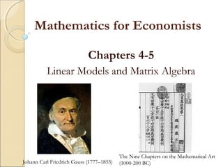
  • 1. Mathematics for Economists Chapters 4-5 Linear Models and Matrix Algebra Johann Carl Friedrich Gauss (1777–1855) The Nine Chapters on the Mathematical Art (1000-200 BC)
  • 2. Objectives of math for economists  To understand mathematical economics problems by stating the unknown, the data and the conditions  To plan solutions to these problems by finding a connection between the data and the unknown  To carry out your plans for solving mathematical economics problems  To examine the solutions to mathematical economics problems for general insights into current and future problems  Remember: Math econ is like love – a simple idea but it can get complicated. 2
  • 3. 4. Linear Algebra  Some history:  The beginnings of matrices and determinants goes back to the second century BC although traces can be seen back to the fourth century BC. But, the ideas did not make it to mainstream math until the late 16th century  The Babylonians around 300 BC studied problems which lead to simultaneous linear equations.  The Chinese, between 200 BC and 100 BC, came much closer to matrices than the Babylonians. Indeed, the text Nine Chapters on the Mathematical Art written during the Han Dynasty gives the first known example of matrix methods.  In Europe, two-by-two determinants were considered by Cardano at the end of the 16th century and larger ones by Leibniz and, in Japan, by Seki about 100 years later.
  • 4. 4. What is a Matrix?  A matrix is a set of elements, organized into rows and columns       dc ba rows columns • a and d are the diagonal elements. • b and c are the off-diagonal elements. • Matrices are like plain numbers in many ways: they can be added, subtracted, and, in some cases, multiplied and inverted (divided).
  • 5. 4. Matrix: Details  Examples: 5 [ ]δβα=      − = b d b A ; 1 1 • Dimensions of a matrix: numbers of rows by numbers of columns. The Matrix A is a 2x2 matrix, b is a 1x3 matrix. • A matrix with only one column or only one row is called a vector. • If a matrix has an equal numbers of rows and columns, it is called a square matrix. Matrix A, above, is a square matrix. • Usual Notation: Upper case letters => matrices Lower case => vectors
  • 6. 4.1 Basic Operations Addition, Subtraction, Multiplication       ++ ++ =      +      hdgc fbea hg fe dc ba       −− −− =      −      hdgc fbea hg fe dc ba       ++ ++ =            dhcfdgce bhafbgae hg fe dc ba Just add elements Just subtract elements Multiply each row by each column       =      kdkc kbka dc ba k Multiply each element by the scalar
  • 7. 4.1 Matrix multiplication: Details  Multiplication of matrices requires a conformability condition  The conformability condition for multiplication is that the column dimensions of the lead matrix A must be equal to the row dimension of the lag matrix B.  What are the dimensions of the vector, matrix, and result? [ ] [ ]131211 232221 131211 1211 cccc bb bbb aaaB ==         = 7 [ ]231213112212121121121111 babababababa +++= • Dimensions: a(1x2), B(2x3) => c(1x3)
  • 8. 4.1 Basic Matrix Operations: Examples 222222 117 25 20 13 97 12 xxx CBA =+       =      +      Matrix addition Matrix subtraction Matrix multiplication Scalar multiplication 8       =      −      65 11 32 01 97 12 222222 x 2726 34 32 01 x 97 12 xxx CBA =       =                  =      8143 2141 16 42 8 1
  • 9. 4.1 Laws of Matrix Addition & Multiplication       ++ ++ =      +      =+ 22222121 12121111 2221 1211 2221 1211 abaa abba bb bb aa aa BA  Commutative law of Matrix Addition: A + B = B + A 9       ++ ++ =      +      =+ 22222121 12121111 2221 1211 2221 1211 abab abab bb aa bb bb AB  Matrix Multiplication is distributive across Additions: A (B+ C) = AB + AC (assuming comformability applies).
  • 10. 4.1 Matrix Multiplication  Matrix multiplication is generally not commutative. That is, AB ≠ BA even if BA is conformable (because diff. dot product of rows or col. of A&B)       − =      = 76 10 , 43 21 BA 10 ( ) ( ) ( ) ( ) ( ) ( ) ( ) ( )       =      +−+ +−+ = 2524 1312 74136403 72116201 AB ( ) ( )( ) ( ) ( ) ( ) ( ) ( ) ( )       −− =      ++ −+−+ = 4027 43 47263716 41203110 BA
  • 11. 4.1 Matrix multiplication  Exceptions to non-commutative law: AB=BA iff B = a scalar, B = identity matrix I, or B = the inverse of A -i.e., A-1 11  Theorem: It is not true that AB = AC => B=C Proof:           −−−=           − =           −− −= 132 111 212 ; 011 010 111 ; 321 101 121 CBA Note: If AB = AC for all matrices A, then B=C.
  • 12. 4.1 Transpose Matrix           − =′=>      − = 49 08 13 401 983 AA:Example  The transpose of a matrix A is another matrix AT (also written A ′) created by any one of the following equivalent actions: - write the rows (columns) of A as the columns (rows) of AT - reflect A by its main diagonal to obtain AT  Formally, the (i,j) element of AT is the (j,i) element of A: [AT ]ij = [A]jj  If A is a m × n matrix => AT is a n × m matrix.  (A')' = A  Conformability changes unless the matrix is square. 12
  • 13. 4.1 Inverse of a Matrix  Identity matrix: AI = A           = 100 010 001 I Notation: Ij is a jxj identity matrix.  Given A (mxn), the matrix B (nxm) is a right-inverse for A iff AB = Im  Given A (mxn), the matrix C (mxn) is a left-inverse for A iff CA = In
  • 14. 4.1 Inverse of a Matrix  Inversion is tricky: (ABC)-1 = C-1 B-1 A-1  More on this topic later  Theorem: If A (mxm), has both a right-inverse B and a left-inverse C, thenC = B. Proof: AB=Im and CA=In. Thus, C(AB)=C Im = C and C(AB)=(CA)B=InB=B => C(nxm)=B(mxn) Note: - This matrix is unique. - If A has both a right and a left inverse, it is called invertible.
  • 15. 4.1 Vector multiplication: Geometric interpretation  Think of a vector as a directed line segment in N- dimensions! (has “length” and “direction”)  Scalar multiplication (“scales” the vector –i.e., changes length)  Source of linear dependence 15 [ ]6 4 2= U [ ]3 2 = U [ ]− ⋅ = − −1 3 2U x2 x1 -4 -3 -2 -1 1 2 3 4 5 6 6 5 4 3 2 1 -2
  • 16. 4.1 Vector Addition: Geometric interpretation  v' = [2 3]  u' = [3 2]  w’= v'+u' = [5 5]  Note that two vectors plus the concepts of addition and multiplication can create a two-dimensional space. 16 x1 x2 5 4 3 2 1 1 2 3 4 5 w u v u A vector space is a mathematical structure formed by a collection of vectors, which may be added together and multiplied by scalars. (It’s closed under multiplication and addition).
  • 17. 4.1 Vector Space  Given a field R and a set V of objects, on which “vector addition” (VxV→V), denoted by “+”, and “scalar multiplication” (RxS →V), denoted by “. ”, are defined. If the following axioms are true for all objects u, v, and w in V and all scalars c and k in R, then V is called a vector space and the objects in V are called vectors. 1. u+v  is in V (closed under addition). 2. u + v = v + u (vector addition is commutative). 3. θ is in V, such that u+ θ = u (null element). 4. u + (v+w) = (v + u) +w (distributive law of vector addition) 5. For each v, there is a –v, such that v+(-v) = θ 6. c .u is in V (closed under scalar multiplication). 7. c. (k . u) = (c .k) u (scalar multiplication is associative).17
  • 18. 4.1 Vector Space 8. c. (v+ u) = (c. v)+ (c. u) 9. (c+k) . u = (c. u)+ (k. u) 10. 1.u=u (unit element). 11. 0.u= θ (zero element). We can write S = {V,R,+,.}to denote an abstract vector space. This is a general definition. If the field R represents the real numbers, then we define a real vector space.  Definition: Linear Combination Given vectors u1,...,uk,, the vector w = c1 u1+....+ ckuk is called a linear combination of the vectors u ,...,u . 18
  • 19. 4.1 Vector Space  Definition: Subspace Given the vector space V and W a sect of vectors, such that W is in V. Then W is a subspace iff: u, v are in W => u+v are in W, and c u is in W for every c in R. u1,...,uk,, the vector w = c1 u1+....+ ckuk is called a linear combination of the vectors u1,...,uk,. 19
  • 20. 4.1 System of equations: Matrices and4.1 System of equations: Matrices and VectorsVectors Assume an economic model as system of linear equations in which aij parameters, where i = 1.. n rows, j = 1.. m columns, and n=m xi endogenous variables, di exogenous variables and constants nn n n nm m m nn d d d x x x ax ax ax axa axa axa       2 1 2 22 12 211 22121 12111 = = = + + + + + + 20
  • 21.  A general form matrix of a system of linear equations Ax = d where A = matrix of parameters x = column vector of endogenous variables d = column vector of exogenous variables and constants  Solve for x* dAx dAx d d d x x x aaa aaa aaa nnnmnn m m 1* 2 1 2 1 21 22221 11211 − = =             =                              21 4.1 System of equations: Matrices and4.1 System of equations: Matrices and VectorsVectors
  • 22. 4.1 Solution of a General-equation System  Assume the 2x2 model 2x + y = 12 4x + 2y = 24 Find x*, y*: y = 12 – 2x 4x + 2(12 – 2x) = 24 4x +24 – 4x = 24 0 = 0 ? indeterminante!  Why? 4x + 2y =24 2(2x + y) = 2(12)  one equation with two unknowns 2x + y = 12 x, y Conclusion: not all simultaneous equation models have solutions (not all matrices have inverses). 22
  • 23. 4.1 Linear dependence  A set of vectors is linearly dependent if any one of them can be expressed as a linear combination of the remaining vectors; otherwise, it is linearly independent.  Formal definition: Linear independent The set {u1,...,uk} is called a linearly independent set of vectors iff c1 u1+....+ ckuk = θ => c1= c2=...=ck,=0.  Notes: - Dependence prevents solving a system of equations. More unknowns than independent equations. - The number of linearly independent rows or columns in a matrix is the rank of a matrix (rank(A)). 23
  • 24. 4.1 Linear dependence  Examples: [ ] [ ] // 2 / 1 ' 2 ' 1 ' 2 ' 1 02 2412 105 2410 125 =−         =      = = vv v v v v 24 [ ] [ ] [ ] 023 54 162216 23 5 4 ; 8 1 ; 7 2 321 3 21 321 =−− == −= −       =      =      = vvv v vv vvv
  • 25. 4.2 Application 1: One Commodity Market Model (2x2 matrix) Economic Model 1) Qd = a – bP (a,b >0) 2) Qs = -c + dP (c,d >0) 3) Qd= Qs  Find P* and Q* Scalar Algebra form (Endogenous Vars :: Constants) 4) 1Q + bP = a 5) 1Q – dP = -c 25 db bcad Q db ca P + − = + + = * *
  • 26. 4.2 One Commodity Market Model (2x2 matrix) 26 dAx c a d b P Q dAx c a P Q d b 1* 1 * * 1 1 1 1 − − =       −      − =      =       − =            − Matrix algebra
  • 27. 4.2 Application II: Three Equation4.2 Application II: Three Equation National Income Model (3x3 matrix)National Income Model (3x3 matrix)  Model Y = C + I0 + G0 C = a + b (Y-T) (a > 0, 0<b<1) T = d + t Y (d > 0, 0<t<1)  Endogenous variables?  Exogenous variables?  Constants?  Parameters?  Why restrictions on the parameters? 27
  • 28. 4.2 Three Equation National Income4.2 Three Equation National Income ModelModel Endogenous: Y, C, T: Income (GNP), Consumption, and Taxes.  Exogenous: I0 and G0: autonomous Investment & Government spending.  Parameters: a & d: autonomous consumption and taxes. t: marginal propensity to tax gross income 0 < t < 1. b: marginal propensity to consume private goods and services from gross income 0 < b < 1.  Solution: 28 btb GIbda Y +− ++− = 1 00*
  • 29. 4.2 Three Equation National Income Model Parameters & Endogenous vars. Exog. vars. Y C T &cons. 1Y -1C +0T = I0+G0 -bY +1C +bT = a -tY +0C +1T = d  Given (Model) Y = C + I0 + G0 C = a + b (Y-T) T = d + t Y  Find Y*, C*, T* 29           + =                     − − − d a GI T C Y t bb 00 10 1 011 dAx dAx 1* − = =
  • 30. 4.2 Three Equation National Income Model 30 dAx d a GI t bb T C Y dAx d a GI T C Y t bb 1* 00 1 * * * 00 10 1 011 10 1 011 − − =           +           − − − =           =           + =                     − − −
  • 31. 4.3 Notes on Vector Operations       = 2 3 12x u An [m x 1] column vector u and a [1 x n] row vector v, yield a product matrix uv of dimension [m x n]. 31 [ ]541 31 =′ x v [ ]       =      =′ 10 15 8 12 2 3 541 2 3 32x vu
  • 32. 4.3 Vector multiplication: Dot (inner), and cross product • The dot product produces a scalar! c’z =1x1=1x4 4x1= z’c 32 44332211 zczczczcy +++= ∑= = 4 1i ii zcy [ ] zc' 4 3 2 1 4321 =             = z z z z ccccy
  • 33. 4.3 Vectors: Dot Product [ ] cfbead f e d cbaT ++=           ==⋅ αββα ccbbaaT ++== 2/1 ][ααα )cos(θβαβα =⋅ Think of the dot product as a matrix multiplication The magnitude (length) is the square root of the dot product of a vector with itself. The dot product is also related to the angle between the two vectors – but it doesn’t tell us the angle. Note: As the cos(90) is zero, the dot product of two orthogonal vectors is zero.
  • 34. 4.3 Vectors: Magnitude and Phase (direction) x y ||v|| θ Alternate representations: Polar coords: (||v||, θ) Complex numbers: ||v||ejθ “phase” runit vectoais,1If 1 2 ),, 2 , 1 ( vv n i i xv n xxxv = = = = ∑  T (Magnitude or “2-norm”) (unit vector => pure direction)
  • 35. 4.3 Vectors: Cross Product  The cross product of vectors A and B is a vector C which is perpendicular to A and B  The magnitude of C is proportional to the cosine of the angle between A and B  The direction of C follows the right hand rule – this why we call it a “right-handed coordinate system” )sin(θbaba =×
  • 36. 4.3 Vectors: Cross Product: Right hand rule
  • 37. 4.3 Vectors: Norm • Given a vector space V, the function g: V→ R is called a norm if and only if: 1) g(x)≥ 0, for all xεV 2) g(x)=0 iff x=θ (empty set) 3) g(αx) = |α|g(x) for all αεR, xεV 4) g(x+y)=g(x)+g(y) (“triangle inequality”) for all x,yεV The norm is a generalization of the notion of size or length of a vector. • An infinite number of functions can be shown to qualify as norms. For vectors in Rn , we have the following examples: g(x)=maxi (xi), g(x)=∑i |xi|, g(x)=[∑i (xi)4 ] ¼ • Given a norm on a vector space, we can define a measure of “how far apart” two vectors are using the concept of a metric.
  • 38. 4.3 Vectors: Metric • Given a vector space V, the function d: VxV→ R is called a metric if and only if: 1) d(x,y)≥ 0, for all x,yεV 2) d(x,y)=0 iff x=y 3) d(x,y) = d(y,x) for all x,yεV 4) d(x+y)≤d(x,z) + d(z,y) (“triangle inequality”) for all x,y,zεV Given a norm g(.), we can define a metric by the equation: d(x,y) = g(x-y). • The dot product is called the Euclidian distance metric.
  • 39. 4.3 Orthonormal Basis  Basis: a space is totally defined by a set of vectors – any point is a linear combination of the basis  Ortho-Normal: orthogonal + normal  Orthogonal: dot product is zero  Normal: magnitude is one  Example: X, Y, Z (but don’t have to be!) [ ] [ ] [ ]T T T z y x 100 010 001 = = = 0 0 0 =⋅ =⋅ =⋅ zy zx yx • X, Y, Z is an orthonormal basis. We can describe any 3D point as a linear combination of these vectors.
  • 40. 4.3 Orthonormal Basis           ⋅+⋅+⋅ ⋅+⋅+⋅ ⋅+⋅+⋅ =                     ncnbna vcvbva ucubua nvu nvu nvu c b a 333 222 111 00 00 00 (not an actual formula – just a way of thinking about it) • To change a point from one coordinate system to another, compute the dot product of each coordinate row with each of the basis vectors. • How do we express any point as a combination of a new basis U, V, N, given X, Y, Z?
  • 41. 4.5 Identity and Null Matrices                           000 000 000 . 100 010 001 10 01 etc or Identity Matrix is a square matrix and also it is a diagonal matrix with 1 along the diagonals. Similar to scalar “1”  Null matrix is one in which all elements are zero. Similar to scalar “0”  Both are diagonal matrices  Both are idempotent matrices: A = AT and A = A2 = A3 = … 41
  • 42. 4.6 Inverse matrix  AA-1 = I  A-1 A=I  Necessary for matrix to be square to have unique inverse  If an inverse exists for a square matrix, it is unique  (A')-1 =(A-1 )' 42 • A x = d • A-1 A x = A-1 d • Ix = A-1 d • x = A-1 d • Solution depends on A-1 • Linear independence • Determinant test!
  • 43. 4.6 Inverse of a Matrix           100 010 001 | ihg fed cba 1. Append the identity matrix to A 2. Subtract multiples of the other rows from the first row to reduce the diagonal element to 1 3. Transform the identity matrix as you go 4. When the original matrix is the identity, the identity has become the inverse!
  • 44. 4.6 Determination of the Inverse (Gauss-Jordan Elimination) AX = I I X = K I X = X = A-1 K = A-1 1) Augmented matrix all A, X and I are (nxn) square matrices X = A-1 Gauss elimination Gauss-Jordan eliminationU: upper triangular further row operations [A I ] [ U H] [ I K] 2) Transform augmented matrix
  • 45. 4.6 Determinant of a Matrix  The determinant is a number associated with any squared matrix.  If A is an nxn matrix, the determinant is given by |A| or det(A).  Determinants are used to characterize invertible matrices. A matrix is invertible (non-singular) if and only if it has a non- zero determinant  That is, if |A|≠0 → A is invertible.  Determinants are used to describe the solution to a system of linear equations with Cramer's rule.  Can be found using factorials, pivots, and cofactors! More on this later.  Lots of interpretations 45
  • 46. 4.6 Determinant of a Matrix  Used for inversion. Example: Inverse of a 2x2 matrix:       = dc ba A bcadAA −== )det(||       − − − =− ac bd bcad A 11 This matrix is called the adjugate of A (or adj(A)). A-1 = adj(A)/|A|
  • 47. 4.6 Determinant of a Matrix (3x3) cegbdiafhcdhbfgaei ihg fed cba −−−++= ihg fed cba ihg fed cba ihg fed cba Sarrus’ Rule: Sum from left to right. Then, subtract from right to left Note: N! terms
  • 48. 4.6 Determinants: Laplace formula  The determinant of a matrix of arbitrary size can be defined by the Leibniz formula or the Laplace formula.  The Laplace formula (or expansion) expresses the determinant | A| as a sum of n determinants of (n-1) × (n-1) sub-matrices of A. There are n2 such expressions, one for each row and column of A  Define the i,j minor Mij (usually written as |Mij|) of A as the determinant of the (n-1) × (n-1) matrix that results from deleting the i-th row and the j-th column of A. 48 Pierre-Simon Laplace (1749–1827).
  • 49. 4.6 Determinants: Laplace formula  Define the Ci,jthe cofactor of A as: 49 ||)1( ,, ji ji ji MC + −= • The cofactor matrix of A -denoted by C-, is defined as the nxn matrix whose (i,j) entry is the (i,j) cofactor of A. The transpose of C is called the adjugate or adjoint of A (adj(A)). • Theorem (Determinant as a Laplace expansion) Suppose A = [aij] is an nxn matrix and i,j= {1, 2, ...,n}. Then the determinant njnjjjijij ininiiii CaCaCa CaCaCaA +++= +++= ... ...|| 22 2211
  • 50. 4.6 Determinants: Laplace formula  Example: 50           −= 642 010 321 A 0)0(x4)3x2-x61)(1()0(x2 0))2x)1((x3)0(x)1(x2)6x1(x1 x3x2x1|| 131211 =−+−+−= =−−+−+−= =++= CCCA  |A| is zero => The matrix is non-singular. (Check!)
  • 51. 4.6 Determinants: Properties  Interchange of rows and columns does not affect |A|. (Corollary, |A| = |A’|.)  |kA| = kn |A|, where k is a scalar.  |I| = 1, where I is the identity matrix.  |A| = |A’|.  |AB| = |A||B|.  |A-1 |=1/|A|. 51
  • 52. 4.6 Matrix inversion: Note  It is not possible to divide one matrix by another. That is, we can not write A/B. For two matrices A and B, the quotient can be written as AB-1 or B-1 A.  In general, in matrix algebra AB-1 ≠ B-1 A. Thus, writing A/B does not clearly identify whether it represents AB-1 or B-1 A. We’ll say B-1 post-multiplies A (for AB-1 ) and B-1 pre-multiplies A (for B-1 A)  Matrix division is matrix inversion. 52
  • 53. 4.7 Application IV: Finite Markov Chains Markov processes are used to measure movements over time. 53 [ ] [ ] [ ] [ ] [ ] [ ] [ ] [ ]90110 100*6.100*3.,100*4.100*7. 6.4. 3.7. 100100 PP PP x plant?eachatbewillemployeesmanyhowyear,oneofendAt the 6.4. 3.7. PP PP M yprobabilitknownaw/plantseachbetweenmoveandstayemployeesThe 100100x B&Aplantsover twoddistributeare0at timeEmployees 0000 BBBA ABAA 00 / 011 BBBA ABAA 00 / 0 = ++=      = ++=      ==       =      = == BBABBAAA PBPBPAPABAMBA BA
  • 54. 4.7 Application IV: Finite Markov Chains  Associative law of multiplication 54 [ ] [ ] [ ] [ ] [ ] [ ] [ ] [ ]8711390*6.110*3.90*4.110*7. 6.4. 3.7. 90110 PP PP PP PP x 90110 PP PP x plant?eachatbewillemployeesmanyhowyears,twoofendAt the BBBA ABAA BBBA ABAA 00 2/ 022 BBBA ABAA 00 / 011 =++=      =             == =      == BAMBA BAMBA
  • 55. Ch. 4 Linear Models & Matrix Algebra: Summary  Matrix algebra can be used: a. to express the system of equations in a compact notation; b. to find out whether solution to a system of equations exist; and c. to obtain the solution if it exists. Need to invert the A matrix to find the solution for x* 55 d A adjA x A adjA A dAx dAx = = = = − − * 1 1* det
  • 56. Ch. 4 Notation and Definitions: Summary  A (Upper case letters) = matrix  b (Lower case letters) = vector  nxm = n rows, m columns  rank(A) = number of linearly independent vectors of A  trace(A) = tr(A) = sum of diagonal elements of A  Null matrix = all elements equal to zero.  Diagonal matrix = all non-zero elements are in the diagonal.  I = identity matrix (diagonal elements: 1, off-diagonal:0)  |A| = det(A) = determinant of A  A-1 = inverse of A  A’=AT = Transpose of A  A=AT Symmetric matrix  A=A-1 Orthogonal matrix |Mij|= Minor of A 56
  • 57.
  • 58. You know too much linear algebra when... You look at the long row of milk cartons at Whole Foods --soy, skim, .5% low-fat, 1% low-fat, 2% low-fat, and whole-- and think: "Why so many? Aren't soy, skim, and whole a basis?"

Editor's Notes

  1. Numerical examples are demonstrated on black board