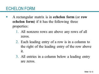
The document provides an overview of matrix theory, including:
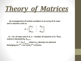
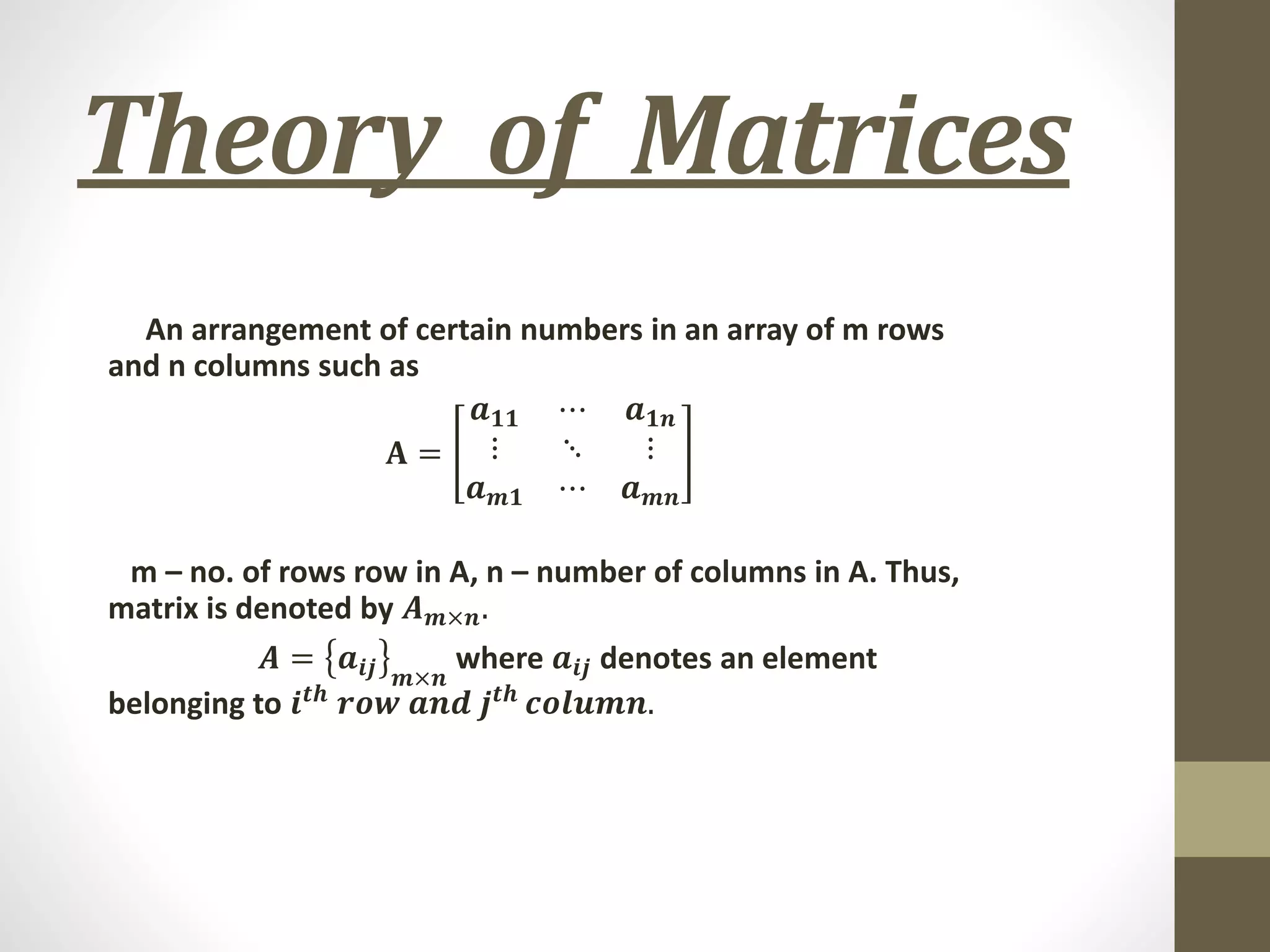
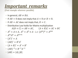
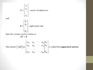
1. The definition and notation of matrices, including that a matrix A is represented as Am×n, where m is the number of rows and n is the number of columns.
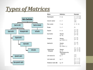
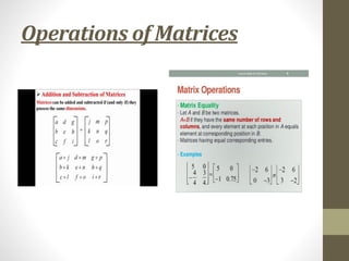
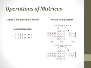
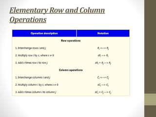
2. The different types of matrices and operations that can be performed on matrices, such as scalar multiplication, matrix multiplication, and properties like the distributive law.
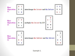
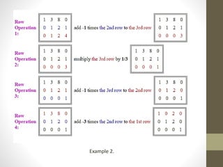
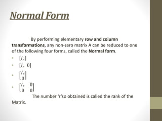
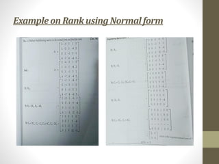
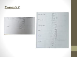
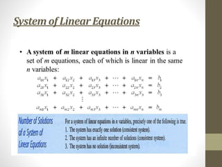
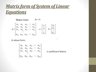
3. Methods for solving systems of linear equations using matrices, including writing the system in matrix form, reducing the augmented matrix to echelon form, and determining the solution based on the rank.
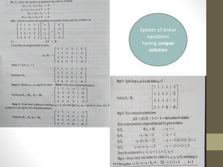
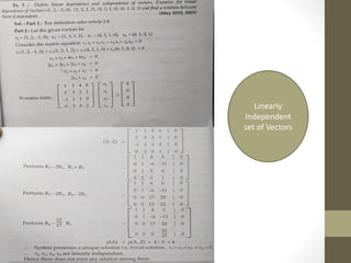
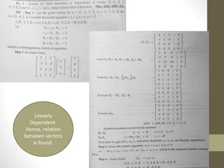
![Solution of System AX=B(Method)
1. Write the given system in matrix form(AX=B).
2. Consider the augmented matrix[A|B] from the given system.
3. Reduce the augmented matrix to the Echelon form.
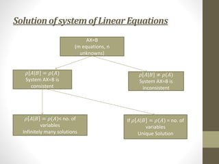
4. Conclude the system has unique, infinite or no solution.
5. If consistent with 𝜌 𝐴 𝐵 = 𝜌 𝐴 = no. of variables then
rewrite equations and find values.
6. If consistent with 𝜌 𝐴 𝐵 = 𝜌 𝐴 = 𝑟 < no. of variables
then put 𝑛 − 𝑟 variables(free variables) as u, v, w etc. find
values of other variables in terms of free variables.
Note : In [A|B], first part represents 𝜌 𝐴 and whole matrix represents
𝜌 𝐴 𝐵 .](https://image.slidesharecdn.com/module1theoryofmatrices-221006111108-ae3904bd/85/Module-1-Theory-of-Matrices-pdf-19-320.jpg)