Linear Algebra and Matrices
Methods for Dummies
21st October, 2009
Elvina Chu & Flavia Mancini
Talk Outline
• Scalars, vectors and matrices
• Vector and matrix calculations
• Identity, inverse matrices & determinants
• Solving simultaneous equations
• Relevance to SPM
Linear Algebra & Matrices, MfD 2009
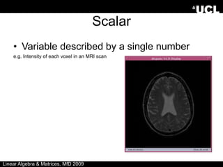
Scalar
• Variable described by a single number
e.g. Intensity of each voxel in an MRI scan
Linear Algebra & Matrices, MfD 2009
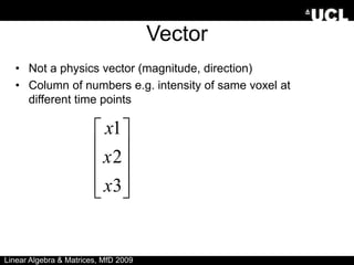
Vector
• Not a physics vector (magnitude, direction)
• Column of numbers e.g. intensity of same voxel at
different time points
Linear Algebra & Matrices, MfD 2009










3
2
1
x
x
x
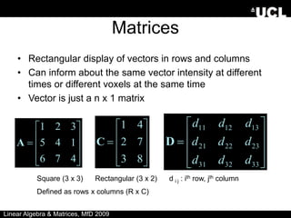
Matrices
• Rectangular display of vectors in rows and columns
• Can inform about the same vector intensity at different
times or different voxels at the same time
• Vector is just a n x 1 matrix











4
7
6
1
4
5
3
2
1
A
Square (3 x 3) Rectangular (3 x 2) d i j : ith row, jth column
Defined as rows x columns (R x C)











8
3
7
2
4
1
C











33
32
31
23
22
21
13
12
11
d
d
d
d
d
d
d
d
d
D
Linear Algebra & Matrices, MfD 2009
Matrices in Matlab
• X=matrix
• ;=end of a row
• :=all row or column










9
8
7
6
5
4
3
2
1
Subscripting – each element of a matrix
can be addressed with a pair of numbers;
row first, column second (Roman Catholic)
e.g. X(2,3) = 6
X(3, :) =
X( [2 3], 2) =
 
9
8
7








8
5
“Special” matrix commands:
• zeros(3,1) =
• ones(2) =
• magic(3) =








1
1
1
1










0
0
0
Linear Algebra & Matrices, MfD 2009










2
9
4
7
5
3
6
1
8
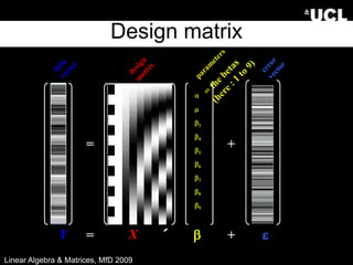
Design matrix
=
a
m
b3
b4
b5
b6
b7
b8
b9
+
e
= b +
Y X ´
Linear Algebra & Matrices, MfD 2009
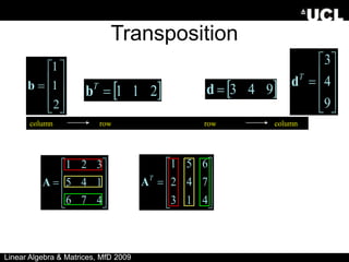
Transposition











2
1
1
b  
2
1
1

T
b  
9
4
3

d
column row row column











4
7
6
1
4
5
3
2
1
A











4
1
3
7
4
2
6
5
1
T
A
Linear Algebra & Matrices, MfD 2009











9
4
3
T
d
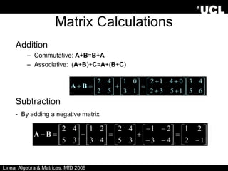
Matrix Calculations
Addition
– Commutative: A+B=B+A
– Associative: (A+B)+C=A+(B+C)
Subtraction
- By adding a negative matrix
































6
5
4
3
1
5
3
2
0
4
1
2
1
3
0
1
5
2
4
2
B
A
Linear Algebra & Matrices, MfD 2009
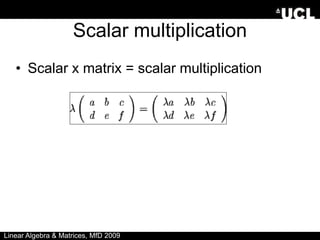
Scalar multiplication
• Scalar x matrix = scalar multiplication
Linear Algebra & Matrices, MfD 2009
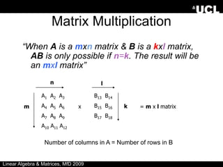
Matrix Multiplication
“When A is a mxn matrix & B is a kxl matrix,
AB is only possible if n=k. The result will be
an mxl matrix”
A1 A2 A3
A4 A5 A6
A7 A8 A9
A10 A11 A12
m
n
x
B13 B14
B15 B16
B17 B18
l
k
Number of columns in A = Number of rows in B
= m x l matrix
Linear Algebra & Matrices, MfD 2009
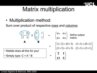
Matrix multiplication
• Multiplication method:
Sum over product of respective rows and columns

1 0
2 3





 







1
3
1
2








22
21
12
11
c
c
c
c


















1)
(3
1)
(2
3)
(3
2)
(2
1)
(0
1)
(1
3)
(0
2)
(1








5
13
1
2
X =
=
=
Define output
matrix
A B
• Matlab does all this for you!
• Simply type: C = A * B
Linear Algebra & Matrices, MfD 2009
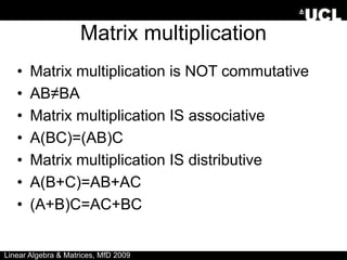
Matrix multiplication
• Matrix multiplication is NOT commutative
• AB≠BA
• Matrix multiplication IS associative
• A(BC)=(AB)C
• Matrix multiplication IS distributive
• A(B+C)=AB+AC
• (A+B)C=AC+BC
Linear Algebra & Matrices, MfD 2009
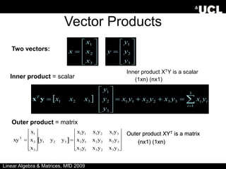
Vector Products
Inner product XTY is a scalar
(1xn) (nx1)
Outer product XYT is a matrix
(nx1) (1xn)
xyT

x1
x2
x3










y1 y2 y3
 
x1y1 x1y2 x1y3
x2y1 x2y2 x2y3
x3y1 x3y2 x3y3










  i
i
i
T
y
x
y
x
y
x
y
x
y
y
y
x
x
x 
















3
1
3
3
2
2
1
1
3
2
1
3
2
1
y
x
Inner product = scalar
Two vectors:











3
2
1
x
x
x
x











3
2
1
y
y
y
y
Outer product = matrix
Linear Algebra & Matrices, MfD 2009
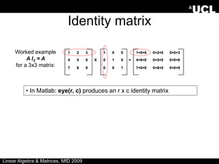
Identity matrix
Is there a matrix which plays a similar role as the number 1 in number
multiplication?
Consider the nxn matrix:
For any nxn matrix A, we have A In = In A = A
For any nxm matrix A, we have In A = A, and A Im = A (so 2 possible matrices)
Linear Algebra & Matrices, MfD 2009
Identity matrix
1 2 3 1 0 0 1+0+0 0+2+0 0+0+3
4 5 6 X 0 1 0 = 4+0+0 0+5+0 0+0+6
7 8 9 0 0 1 7+0+0 0+8+0 0+0+9
Worked example
A I3 = A
for a 3x3 matrix:
• In Matlab: eye(r, c) produces an r x c identity matrix
Linear Algebra & Matrices, MfD 2009
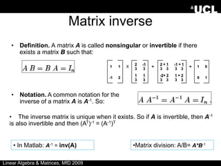
Matrix inverse
• Definition. A matrix A is called nonsingular or invertible if there
exists a matrix B such that:
• Notation. A common notation for the
inverse of a matrix A is A-1. So:
• The inverse matrix is unique when it exists. So if A is invertible, then A-1
is also invertible and then (AT)-1 = (A-1)T
1 1 X
2
3
-1
3
=
2 + 1
3 3
-1 + 1
3 3
= 1 0
-1 2
1
3
1
3
-2+ 2
3 3
1 + 2
3 3
0 1
• In Matlab: A-1 = inv(A) •Matrix division: A/B= A*B-1
Linear Algebra & Matrices, MfD 2009
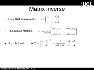
Matrix inverse
• For a XxX square matrix:
• The inverse matrix is:
Linear Algebra & Matrices, MfD 2009
• E.g.: 2x2 matrix
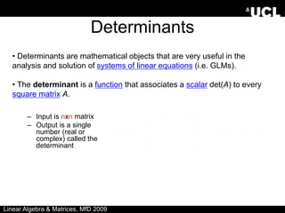
Determinants
• Determinants are mathematical objects that are very useful in the
analysis and solution of systems of linear equations (i.e. GLMs).
• The determinant is a function that associates a scalar det(A) to every
square matrix A.
– Input is nxn matrix
– Output is a single
number (real or
complex) called the
determinant
Linear Algebra & Matrices, MfD 2009
Determinants
•Determinants can only be found for square matrices.
•For a 2x2 matrix A, det(A) = ad-bc. Lets have at closer look at that:
• A matrix A has an inverse matrix A-1 if and only if det(A)≠0.
• In Matlab: det(A) = det(A)
Linear Algebra & Matrices, MfD 2009
a b
c d
det(A) = = ad - bc
[ ]
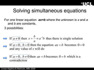
Solving simultaneous equations
For one linear equation ax=b where the unknown is x and a
and b are constants,
3 possibilities:
If 0

a then b
a
a
b
x 1


 thus there is single solution
If 0

a , 0

b then the equation b
ax  becomes 0
0 
and any value of x will do
If 0

a , 0

b then b
ax  becomes b

0 which is a
contradiction
Linear Algebra & Matrices, MfD 2009
With >1 equation and >1 unknown
• Can use solution from the single
equation to solve
• For example
• In matrix form
b
a
x 1


1
2
5
3
2
2
1
2
1





x
x
x
x
A X = B




















 1
5
2
1
3
2
2
1
x
x
X =A-1B
Linear Algebra & Matrices, MfD 2009






4
1
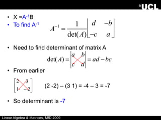
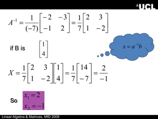
• X =A-1B
• To find A-1
• Need to find determinant of matrix A
• From earlier
(2 -2) – (3 1) = -4 – 3 = -7
• So determinant is -7
bc
ad
d
c
b
a
A 


)
det(






 2
1
3
2
Linear Algebra & Matrices, MfD 2009

A1

1
det(A)
d b
c a


























2
1
3
2
7
1
2
1
3
2
)
7
(
1
1
A
1
2
7
14
7
1
4
1
2
1
3
2
7
1
























X






4
1
if B is
So
b
a
x 1


Linear Algebra & Matrices, MfD 2009
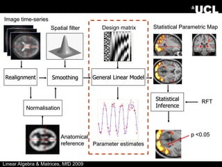
How are matrices relevant
to fMRI data?
Normalisation
Statistical Parametric Map
Image time-series
Parameter estimates
General Linear Model
Realignment Smoothing
Design matrix
Anatomical
reference
Spatial filter
Statistical
Inference
RFT
p <0.05
Linear Algebra & Matrices, MfD 2009
BOLD signal
Time
single voxel
time series
Voxel-wise time series analysis
Model
specification
Parameter
estimation
Hypothesis
Statistic
SPM
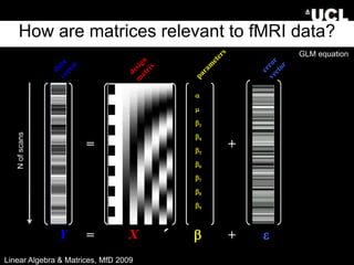
How are matrices relevant to fMRI data?
=
a
m
b3
b4
b5
b6
b7
b8
b9
+
e
= b +
Y X ´
Linear Algebra & Matrices, MfD 2009
GLM equation
N
of
scans
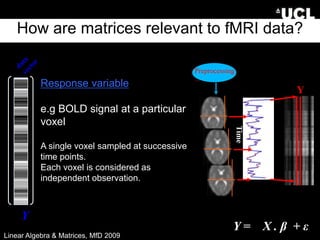
How are matrices relevant to fMRI data?
Y
Response variable
e.g BOLD signal at a particular
voxel
A single voxel sampled at successive
time points.
Each voxel is considered as
independent observation.
Preprocessing
...
Intens
ity
Ti
me
Y
Time
Y = X . β + ε
Linear Algebra & Matrices, MfD 2009
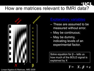
How are matrices relevant to fMRI data?
a
m
b3
b4
b5
b6
b7
b8
b9
b
X ´
Explanatory variables
– These are assumed to be
measured without error.
– May be continuous;
– May be dummy,
indicating levels of an
experimental factor.
Y = X . β + ε
Solve equation for β – tells us
how much of the BOLD signal is
explained by X
Linear Algebra & Matrices, MfD 2009
In Practice
• Estimate MAGNITUDE of signal changes
• MR INTENSITY levels for each voxel at
various time points
• Relationship between experiment and
voxel changes are established
• Calculation and notation require linear
algebra
Linear Algebra & Matrices, MfD 2009
Summary
• SPM builds up data as a matrix.
• Manipulation of matrices enables unknown
values to be calculated.
Y = X . β + ε
Observed = Predictors * Parameters + Error
BOLD = Design Matrix * Betas + Error
Linear Algebra & Matrices, MfD 2009
References
• SPM course http://www.fil.ion.ucl.ac.uk/spm/course/
• Web Guides
http://mathworld.wolfram.com/LinearAlgebra.html
http://www.maths.surrey.ac.uk/explore/emmaspages/option1.ht
ml
http://www.inf.ed.ac.uk/teaching/courses/fmcs1/
(Formal Modelling in Cognitive Science course)
• http://www.wikipedia.org
• Previous MfD slides
Linear Algebra & Matrices, MfD 2009

LinearAlgebra.ppt

  • 1.
    Linear Algebra andMatrices Methods for Dummies 21st October, 2009 Elvina Chu & Flavia Mancini
  • 2.
    Talk Outline • Scalars,vectors and matrices • Vector and matrix calculations • Identity, inverse matrices & determinants • Solving simultaneous equations • Relevance to SPM Linear Algebra & Matrices, MfD 2009
  • 3.
    Scalar • Variable describedby a single number e.g. Intensity of each voxel in an MRI scan Linear Algebra & Matrices, MfD 2009
  • 4.
    Vector • Not aphysics vector (magnitude, direction) • Column of numbers e.g. intensity of same voxel at different time points Linear Algebra & Matrices, MfD 2009           3 2 1 x x x
  • 5.
    Matrices • Rectangular displayof vectors in rows and columns • Can inform about the same vector intensity at different times or different voxels at the same time • Vector is just a n x 1 matrix            4 7 6 1 4 5 3 2 1 A Square (3 x 3) Rectangular (3 x 2) d i j : ith row, jth column Defined as rows x columns (R x C)            8 3 7 2 4 1 C            33 32 31 23 22 21 13 12 11 d d d d d d d d d D Linear Algebra & Matrices, MfD 2009
  • 6.
    Matrices in Matlab •X=matrix • ;=end of a row • :=all row or column           9 8 7 6 5 4 3 2 1 Subscripting – each element of a matrix can be addressed with a pair of numbers; row first, column second (Roman Catholic) e.g. X(2,3) = 6 X(3, :) = X( [2 3], 2) =   9 8 7         8 5 “Special” matrix commands: • zeros(3,1) = • ones(2) = • magic(3) =         1 1 1 1           0 0 0 Linear Algebra & Matrices, MfD 2009           2 9 4 7 5 3 6 1 8
  • 7.
    Design matrix = a m b3 b4 b5 b6 b7 b8 b9 + e = b+ Y X ´ Linear Algebra & Matrices, MfD 2009
  • 8.
    Transposition            2 1 1 b   2 1 1  T b  9 4 3  d column row row column            4 7 6 1 4 5 3 2 1 A            4 1 3 7 4 2 6 5 1 T A Linear Algebra & Matrices, MfD 2009            9 4 3 T d
  • 9.
    Matrix Calculations Addition – Commutative:A+B=B+A – Associative: (A+B)+C=A+(B+C) Subtraction - By adding a negative matrix                                 6 5 4 3 1 5 3 2 0 4 1 2 1 3 0 1 5 2 4 2 B A Linear Algebra & Matrices, MfD 2009
  • 10.
    Scalar multiplication • Scalarx matrix = scalar multiplication Linear Algebra & Matrices, MfD 2009
  • 11.
    Matrix Multiplication “When Ais a mxn matrix & B is a kxl matrix, AB is only possible if n=k. The result will be an mxl matrix” A1 A2 A3 A4 A5 A6 A7 A8 A9 A10 A11 A12 m n x B13 B14 B15 B16 B17 B18 l k Number of columns in A = Number of rows in B = m x l matrix Linear Algebra & Matrices, MfD 2009
  • 12.
    Matrix multiplication • Multiplicationmethod: Sum over product of respective rows and columns  1 0 2 3               1 3 1 2         22 21 12 11 c c c c                   1) (3 1) (2 3) (3 2) (2 1) (0 1) (1 3) (0 2) (1         5 13 1 2 X = = = Define output matrix A B • Matlab does all this for you! • Simply type: C = A * B Linear Algebra & Matrices, MfD 2009
  • 13.
    Matrix multiplication • Matrixmultiplication is NOT commutative • AB≠BA • Matrix multiplication IS associative • A(BC)=(AB)C • Matrix multiplication IS distributive • A(B+C)=AB+AC • (A+B)C=AC+BC Linear Algebra & Matrices, MfD 2009
  • 14.
    Vector Products Inner productXTY is a scalar (1xn) (nx1) Outer product XYT is a matrix (nx1) (1xn) xyT  x1 x2 x3           y1 y2 y3   x1y1 x1y2 x1y3 x2y1 x2y2 x2y3 x3y1 x3y2 x3y3             i i i T y x y x y x y x y y y x x x                  3 1 3 3 2 2 1 1 3 2 1 3 2 1 y x Inner product = scalar Two vectors:            3 2 1 x x x x            3 2 1 y y y y Outer product = matrix Linear Algebra & Matrices, MfD 2009
  • 15.
    Identity matrix Is therea matrix which plays a similar role as the number 1 in number multiplication? Consider the nxn matrix: For any nxn matrix A, we have A In = In A = A For any nxm matrix A, we have In A = A, and A Im = A (so 2 possible matrices) Linear Algebra & Matrices, MfD 2009
  • 16.
    Identity matrix 1 23 1 0 0 1+0+0 0+2+0 0+0+3 4 5 6 X 0 1 0 = 4+0+0 0+5+0 0+0+6 7 8 9 0 0 1 7+0+0 0+8+0 0+0+9 Worked example A I3 = A for a 3x3 matrix: • In Matlab: eye(r, c) produces an r x c identity matrix Linear Algebra & Matrices, MfD 2009
  • 17.
    Matrix inverse • Definition.A matrix A is called nonsingular or invertible if there exists a matrix B such that: • Notation. A common notation for the inverse of a matrix A is A-1. So: • The inverse matrix is unique when it exists. So if A is invertible, then A-1 is also invertible and then (AT)-1 = (A-1)T 1 1 X 2 3 -1 3 = 2 + 1 3 3 -1 + 1 3 3 = 1 0 -1 2 1 3 1 3 -2+ 2 3 3 1 + 2 3 3 0 1 • In Matlab: A-1 = inv(A) •Matrix division: A/B= A*B-1 Linear Algebra & Matrices, MfD 2009
  • 18.
    Matrix inverse • Fora XxX square matrix: • The inverse matrix is: Linear Algebra & Matrices, MfD 2009 • E.g.: 2x2 matrix
  • 19.
    Determinants • Determinants aremathematical objects that are very useful in the analysis and solution of systems of linear equations (i.e. GLMs). • The determinant is a function that associates a scalar det(A) to every square matrix A. – Input is nxn matrix – Output is a single number (real or complex) called the determinant Linear Algebra & Matrices, MfD 2009
  • 20.
    Determinants •Determinants can onlybe found for square matrices. •For a 2x2 matrix A, det(A) = ad-bc. Lets have at closer look at that: • A matrix A has an inverse matrix A-1 if and only if det(A)≠0. • In Matlab: det(A) = det(A) Linear Algebra & Matrices, MfD 2009 a b c d det(A) = = ad - bc [ ]
  • 21.
    Solving simultaneous equations Forone linear equation ax=b where the unknown is x and a and b are constants, 3 possibilities: If 0  a then b a a b x 1    thus there is single solution If 0  a , 0  b then the equation b ax  becomes 0 0  and any value of x will do If 0  a , 0  b then b ax  becomes b  0 which is a contradiction Linear Algebra & Matrices, MfD 2009
  • 22.
    With >1 equationand >1 unknown • Can use solution from the single equation to solve • For example • In matrix form b a x 1   1 2 5 3 2 2 1 2 1      x x x x A X = B                      1 5 2 1 3 2 2 1 x x X =A-1B Linear Algebra & Matrices, MfD 2009       4 1
  • 23.
    • X =A-1B •To find A-1 • Need to find determinant of matrix A • From earlier (2 -2) – (3 1) = -4 – 3 = -7 • So determinant is -7 bc ad d c b a A    ) det(        2 1 3 2 Linear Algebra & Matrices, MfD 2009  A1  1 det(A) d b c a      
  • 24.
  • 25.
    Linear Algebra &Matrices, MfD 2009 How are matrices relevant to fMRI data?
  • 26.
    Normalisation Statistical Parametric Map Imagetime-series Parameter estimates General Linear Model Realignment Smoothing Design matrix Anatomical reference Spatial filter Statistical Inference RFT p <0.05 Linear Algebra & Matrices, MfD 2009
  • 27.
    Linear Algebra &Matrices, MfD 2009 BOLD signal Time single voxel time series Voxel-wise time series analysis Model specification Parameter estimation Hypothesis Statistic SPM
  • 28.
    How are matricesrelevant to fMRI data? = a m b3 b4 b5 b6 b7 b8 b9 + e = b + Y X ´ Linear Algebra & Matrices, MfD 2009 GLM equation N of scans
  • 29.
    How are matricesrelevant to fMRI data? Y Response variable e.g BOLD signal at a particular voxel A single voxel sampled at successive time points. Each voxel is considered as independent observation. Preprocessing ... Intens ity Ti me Y Time Y = X . β + ε Linear Algebra & Matrices, MfD 2009
  • 30.
    How are matricesrelevant to fMRI data? a m b3 b4 b5 b6 b7 b8 b9 b X ´ Explanatory variables – These are assumed to be measured without error. – May be continuous; – May be dummy, indicating levels of an experimental factor. Y = X . β + ε Solve equation for β – tells us how much of the BOLD signal is explained by X Linear Algebra & Matrices, MfD 2009
  • 31.
    In Practice • EstimateMAGNITUDE of signal changes • MR INTENSITY levels for each voxel at various time points • Relationship between experiment and voxel changes are established • Calculation and notation require linear algebra Linear Algebra & Matrices, MfD 2009
  • 32.
    Summary • SPM buildsup data as a matrix. • Manipulation of matrices enables unknown values to be calculated. Y = X . β + ε Observed = Predictors * Parameters + Error BOLD = Design Matrix * Betas + Error Linear Algebra & Matrices, MfD 2009
  • 33.
    References • SPM coursehttp://www.fil.ion.ucl.ac.uk/spm/course/ • Web Guides http://mathworld.wolfram.com/LinearAlgebra.html http://www.maths.surrey.ac.uk/explore/emmaspages/option1.ht ml http://www.inf.ed.ac.uk/teaching/courses/fmcs1/ (Formal Modelling in Cognitive Science course) • http://www.wikipedia.org • Previous MfD slides Linear Algebra & Matrices, MfD 2009