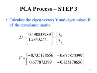
PCA is a dimensionality reduction technique that uses linear transformations to project high-dimensional data onto a lower-dimensional space while retaining as much information as possible. It works by identifying patterns in data and expressing the data in such a way as to highlight their similarities and differences. Specifically, PCA uses linear combinations of the original variables to extract the most important patterns from the data in the form of principal components. The first principal component accounts for as much of the variability in the data as possible, and each succeeding component accounts for as much of the remaining variability as possible.

1. Dimensionality Reduction Introduction
(Dimension Reduction Algorithms, Mathematics for AI & ML ,Semester V)
by
Mr. Rohan Borgalli
(Assistant Professor, Department of Electronics & Telecommunication
Engineering)
Email: rohan.borgalli@sakec.ac.in
SHAH AND ANCHOR KUTCHHI ENGINEERING COLLEGE
DEPARTMENT
OF
ELECTRONICS & TELECOMMUNICATION ENGINEERING

2. Topic Learning Outcomes (TLOs)
Lecture
number
Lecture Contents as per Syllabus Topic Learning
Outcome
Module
No.
Blooms
Level (BL)
Course
Outcome
number
Book No.
Referred
41, 42
Module 6: Dimension
Reduction Algorithms
6.0 Dimension Reduction
Algorithms
6.1 Introduction to Dimension
Reduction Algorithms, Linear
Dimensionality Reduction:
Principal component analysis
To Explain
fundamental of
Dimension
Reduction
6
2:
Understand
HAIMLC5016 T1, T2
HAIMLC5016: Describe Dimension Reduction Algorithms
Text Books:
1. Mathematics for Machine Learning, Marc Peter Deisenroth, A. Aldo Faisal, Cheng Soon Ong,
Cambridge University Press.
2. Exploratory Data Analysis, John Tukey, Princeton University and Bell Laboratories.
Dimension Reduction Algorithms Electronics & Telecommunication Engineering
Mathematics for AI & ML

3. Syllabus
6.0 Dimension Reduction Algorithms
6.1 Introduction to Dimension Reduction
Algorithms, Linear Dimensionality Reduction:
Principal component analysis,
Factor Analysis,
Linear discriminant analysis.
6.2 Non-Linear Dimensionality Reduction:
Multidimensional Scaling,
Isometric Feature Mapping. Minimal polynomial
3

4. Dimensionality Reduction

5. Curse of Dimensionality
Increasing the number of features will not
always improve classification accuracy.
In practice, the inclusion of more features
might actually lead to worse performance.
The number of training examples required
increases exponentially with
dimensionality d (i.e., kd).
32 bins
33 bins
31 bins
k: number of bins per feature
k=3

6. 6
Dimensionality Reduction
What is the objective?
Choose an optimum set of features of lower dimensionality to improve
classification accuracy.
Different methods can be used to reduce dimensionality:
Feature extraction
Feature selection

7. 7
Dimensionality Reduction (cont’d)
Feature extraction: finds a set of new features
(i.e., through some mapping f()) from the
existing features.
1
2
1
2
.
.
.
.
.
.
. K
i
i
i
N
x
x
x
x
x
x
 
 
   
   
   
   
  
   
   
   
   
 
 
 
x y
1
2
1
2
( )
.
.
.
.
.
.
.
f
K
N
x
x
y
y
y
x
 
 
   
   
   
   
 
 
   
   
   
 
 
 
 
 
x
x y
Feature selection:
chooses a subset of the
original features.
The mapping f()
could be linear or
non-linear
K<<N K<<N

8. 1
2
1
2
( )
.
.
.
.
.
.
.
f
K
N
x
x
y
y
y
x
 
 
   
   
   
   
 
 
   
   
   
 
 
 
 
 
x
x y
Feature Extraction
Linear combinations are particularly attractive because they are
simpler to compute and analytically tractable.
Given x ϵ RN, find an K x N matrix T such that:
y = Tx ϵ RK where K<<N
8
T This is a projection from the
N-dimensional space to a K-
dimensional space.

9. Feature Extraction (cont’d)
From a mathematical point of view, finding an optimum mapping
y=𝑓(x) is equivalent to optimizing an objective criterion.
Different methods use different objective criteria, e.g.,
Minimize Information Loss: represent the data as accurately as possible in
the lower-dimensional space.
Maximize Discriminatory Information: enhance the class-discriminatory
information in the lower-dimensional space.
9

10. Feature Extraction (cont’d)
Popular linear feature extraction methods:
Principal Components Analysis (PCA): Seeks a projection that preserves
as much information in the data as possible.
Linear Discriminant Analysis (LDA): Seeks a projection that best
discriminates the data.
Many other methods:
Making features as independent as possible (Independent Component
Analysis or ICA).
Retaining interesting directions (Projection Pursuit).
Embedding to lower dimensional manifolds (Isomap, Locally Linear
Embedding or LLE).
10

11. Vector Representation
A vector x ϵ Rn can be represented by n
components:
Assuming the standard base <v1, v2, …,
vN> (i.e., unit vectors in each
dimension), xi can be obtained by
projecting x along the direction of vi:
x can be “reconstructed” from its
projections as follows:
11
1
2
.
.
:
.
.
.
N
x
x
x
 
 
 
 
 
 
 
 
 
 
 
 
 
x
T
T
i
i i
T
i i
v
x v
v v
 
x
x
1 1 2 2
1
...
N
i i N N
i
x v x v x v x v

    

x
• Since the basis vectors are the same for all x ϵ Rn
(standard basis), we typically represent them as a
n-component vector.

12. Vector Representation (cont’d)
Example assuming n=2:
Assuming the standard base <v1=i,
v2=j>, xi can be obtained by projecting
x along the direction of vi:
x can be “reconstructed” from its
projections as follows:
12
1
2
3
:
4
x
x
   

   
 
 
x
 
1
1
3 4 3
0
T
x i
 
  
 
 
x
3 4
i j
 
x
 
2
0
3 4 4
1
T
x j
 
  
 
 
x
i
j

14. PCA is …
• Abackbone of modern data analysis.
• A black box that is widely used but
poorly understood.
PCA
PCA
OK … let’s dispel the magic behind
this black box

15. PCA - Overview
• It is a mathematical tool from applied linear
algebra.
• It is a simple, non-parametric method of
extracting relevant information from confusing
data sets.
• It provides a roadmap for how to reduce a
complex data set to a lower dimension.

16. Background
• Linear Algebra
• Principal Component Analysis (PCA)
• Independent Component Analysis (ICA)
• Linear Discriminant Analysis (LDA)
• Examples
• Face Recognition - Application

17. 5
• V
ariance is claimed to be the original statistical
measure of spread of data.
n  1
X  X 2
n
 i
i1
 2

Variance
• A measure of the spread of the data in a data
set with mean X

18. Covariance
• Variance – measure of the deviation from the mean for points in one
dimension, e.g., heights
• Covariance – a measure of how much each of the dimensions varies
from the mean with respect to each other.
• Covariance is measured between 2 dimensions to see if there is a
relationship between the 2 dimensions, e.g., number of hours studied
and grade obtained.
• The covariance between one dimension and itself is the variance
X  X 
Y  Y 
n  1
n  1
co v( X ,Y ) 
var( X ) 
n

i1
i i
X  X X  X 
i i
i1

19. 19
Covariance
• What is the interpretation of covariance calculations?
• Say you have a 2-dimensional data set
– X: number of hours studied for a subject
– Y: marks obtained in that subject
• And assume the covariance value (between X and Y) is:
104.53
• What doesthisvaluemean?

20. 20
Covariance
• Exact value is not as important as its sign.
• A positive value of covariance indicates that both
dimensions increase or decrease together, e.g., as the
number of hours studied increases, the grades in that
subject also increase.
• A negative value indicates while one increases the other
decreases, or vice-versa, e.g., active social life vs.
performance in ECE Dept.
• If covariance is zero: the two dimensions are independent
of each other, e.g., heights of students vs. grades obtained
in a subject.

21. 21
Covariance
• Why bother with calculating (expensive)
covariance when we could just plot the 2 values
to see their relationship?
Covariance
relationships
calculations
between
are used
dimensions
to find
in high
dimensional data sets (usually greater than 3)
where visualization is difficult.

22. 22
Covariance Matrix
• Representing covariance among dimensions as a
matrix, e.g., for 3 dimensions:
– Diagonal: variances of the variables
– cov(X,Y)=cov(Y,X), hence matrix is symmetrical about
the diagonal (upper triangular)
– m-dimensional data will result in mxm covariance matrix


cov(Z, X )
• Properties:

cov(Z,Z)

cov(Y,Z)
cov(X,Z)
C  cov(Y, X )
cov(X, X ) cov(X,Y)
cov(Y,Y)
cov(Z,Y)

23. Linear algebra
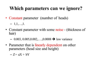
• MatrixA:
• Matrix Transpose
• Vector a
a1 

 

mn 
... 
...
a ... a
 ... ... ...
a a ... a
ij mn
A [a ]
m2
 m1
2n 
22
21
a1n 
a11 a12
a
1 i  n,1 j  m
B [b ]  AT
 b  a ;
ij nm ij ji
 [a1,...,an ]
aT
 

an 

a  ...;

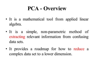
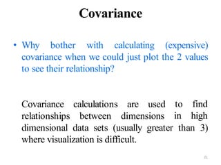
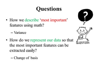
24. Matrix and vector multiplication
• Matrix multiplication
A [aij ]mp ; B [bij ]pn ;
AB  C [cij ]mn ,where cij  rowi (A)colj (B)
• Outer vector product
a  A [a ] ; bT
 B [b ] ;
ij m1 ij 1n
c ab  AB,an mn matrix
• Vector-matrix product
A [aij ]mn ; b  B [bij ]n1;
C  Ab  an m1matrix  vector of length m

25. Inner Product
• Inner (dot) product:
• Length (Eucledian norm) of a vector
• a is normalized iff | | a | | = 1
• The angle between two n-dimesional
vectors
• An inner product is a measure of
collinearity:
– a and b are orthogonal iff
– a and b are collinear iff
• Aset of vectors is linearlyindependent if
no vector is a linear combination of
other vectors.
n
T
a b  a b
 i i
i1
n
i
a
a  aT
a  
i1
2
|| a |||| b ||
cos 
aT
b
aT
b  0
aT
b || a |||| b ||

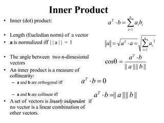
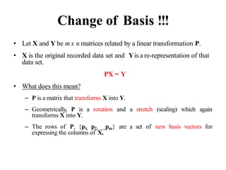
26. Determinant and Trace
• Determinant
• Trace
n
j1
A  (1)i j
det(M )
ij ij
det(AB)= det(A)det(B)
i 1,....n;
A  [aij ]nn ;
det(A)  aij Aij ;
n
A [aij ]nn; tr[A]  ajj
j1

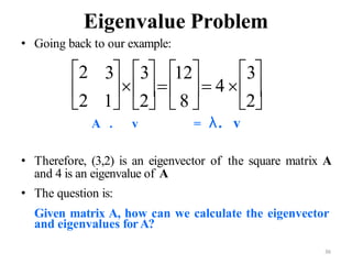
27. Matrix Inversion
• A(n x n) is nonsingular if there exists B such that:
AB  BA  I ; B  A1
n
• A=[2 3; 2 2], B=[-1 3/2; 1 -1]
• Ais nonsingular iff
• Pseudo-inverse for a non square matrix, provided
AT
A is not singular
A#
[AT
A]1
AT
A#
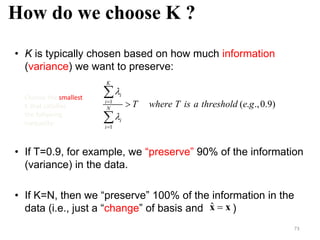
A I
|| A|| 0

28. Linear Independence
• A set of n-dimensional vectors xi Є Rn, are said
to be linearly independent if none of them can
be written as a linear combination of the others.
• In other words,
c1x1  c2 x2  ...  ck xk  0
iff c1  c2  ... ck  0

29. Linear Independence
• Another approach to reveal a
independence is by graphing the vectors.
vectors
 4
6
2
3
2
1
, x   
   
x   
 
  2
3
2
1
2
1 , x   
x   
Not linearly independent vectors Linearly independent vectors

30. Span
• A span of a set of vectors x1, x2, … , xk is the
set of vectors that can be written as a linear
combination of x1, x2, … , xk .
spanx1, x2,...,xk  
c1x1 c2x2 ... ck xk | c1,c2,...,ck 

31. Basis
• A basis for Rn is a set of vectors which:
– Spans Rn , i.e. any vector in this n-dimensional space
can be written as linear combination of these basis
vectors.
– Are linearly independent
• Clearly, any set of n-linearly independent vectors
form basis vectors for Rn.

32. Orthogonal/Orthonormal Basis
• An orthonormal basis of an a vector space V with an inner product, is a set
of basis vectors whose elements are mutually orthogonal and of magnitude 1 (unit
vectors).
• Elements in an orthogonal basis do not have to be unit vectors, but must be mutually
perpendicular. It is easy to change the vectors in an orthogonal basis by scalar
multiples to get an orthonormal basis, and indeed this is a typical way that an
orthonormal basis is constructed.
• Two vectors are orthogonal if they are perpendicular, i.e., they form a right angle, i.e.
if their inner product is zero.
• The standard basis of the n-dimensional Euclidean space Rn is an example of
orthonormal (and ordered) basis.
n
aibi  0  a  b

i1
T
a b 

33. 21
Transformation Matrices
• Consider the following:
• The square (transformation) matrix scales (3,2)
• Now assume we take a multiple of (3,2)
   
3 3 12
   4 
3
2       
2 1 2  8  2
   
      

4 16  4
 2 1
3

6 

24 
 4 
6 
2
   
2 4
2 
3 

6 

34. 34
Transformation Matrices
• Scale vector (3,2) by a value 2 to get (6,4)
• Multiply by the square transformation matrix
• And we see that the result is still scaled by 4.
WHY?
A vector consists of both length and direction. Scaling a
vector only changes its length and not its direction. This is
an important observation in the transformation of matrices
leading to formation of eigenvectors and eigenvalues.
Irrespective of how much we scale (3,2) by, the solution
(under the given transformation matrix) is always a multiple
of 4.

35. 35
Eigenvalue Problem
• The eigenvalue problem is any problem having the
following form:
A. v = λ. v
A: m x m matrix
v: mx 1 non-zero vector
λ: scalar
• Any value of λ for which this equation has a
solution is called the eigenvalue of A and the vector
v which corresponds to this value is called the
eigenvector of A.

36. 36
Eigenvalue Problem
• Going back to our example:
A . v = λ. v
• Therefore, (3,2) is an eigenvector of the square matrix A
and 4 is an eigenvalue of A
• The question is:
Given matrix A, how can we calculate the eigenvector
and eigenvalues forA?
1 2
   
3 3 12
   4 
3
2       
2  8  2
   

37. 37
Calculating Eigenvectors & Eigenvalues
• Simple matrix algebra shows that:
A. v = λ. v
 A. v - λ. I . v = 0
 (A- λ. I ). v = 0
• Finding the roots of | A - λ . I| will give the eigenvalues
and for each of these eigenvalues there will be an
eigenvector
Example …

38. Calculating Eigenvectors &
Eigenvalues
• Let
• And setting the determinant to 0, we obtain 2 eigenvalues:
λ1 = -1 and λ2 = -2
• Then:
A .I 
 
38

  3   21 2
 3  2
 2 3 

  1
    

 0 1  1 0   0 1   0
 2 3  0 1

 2 3  0 

A 

 0 1 
2 3




39. 39
Calculating Eigenvectors & Eigenvalues
• For λ1the eigenvector is:
A  1.I .v1  0
• Therefore the first eigenvector is any column vector in
which the two elements have equal magnitude and opposite
sign.
v1:1 v1:2  0
v1:1  v1:2
and  2v1:1  2v1:2  0
  0
1  v1:1 
   1:2 
 2  2.v
 1

40. 40
Calculating Eigenvectors & Eigenvalues
• Therefore eigenvector v1 is
where k1 is some constant.
• Similarly we find that eigenvector v2
2
where k is some constant.
 
 
1
1 1
v  k
1
 
 
 2
2 2
v  k
1

41. 29
Properties of Eigenvectors and
Eigenvalues
• Eigenvectors can only be found for square matrices and
not every square matrix has eigenvectors.
• Given an m x m matrix (with eigenvectors), we can find
neigenvectors.
• All eigenvectors of a symmetric* matrix are
perpendicular to each other, no matter how many
dimensions we have.
• In practice eigenvectors are normalized to have unit
length.
*Note: covariance matrices are symmetric!

42. Vector Representation
A vector x ϵ Rn can be represented by n
components:
Assuming the standard base <v1, v2, …,
vN> (i.e., unit vectors in each
dimension), xi can be obtained by
projecting x along the direction of vi:
x can be “reconstructed” from its
projections as follows:
42
1
2
.
.
:
.
.
.
N
x
x
x
 
 
 
 
 
 
 
 
 
 
 
 
 
x
T
T
i
i i
T
i i
v
x v
v v
 
x
x
1 1 2 2
1
...
N
i i N N
i
x v x v x v x v

    

x
• Since the basis vectors are the same for all x ϵ Rn
(standard basis), we typically represent them as a
n-component vector.

43. Vector Representation (cont’d)
Example assuming n=2:
Assuming the standard base <v1=i,
v2=j>, xi can be obtained by projecting
x along the direction of vi:
x can be “reconstructed” from its
projections as follows:
43
1
2
3
:
4
x
x
   

   
 
 
x
 
1
1
3 4 3
0
T
x i
 
  
 
 
x
3 4
i j
 
x
 
2
0
3 4 4
1
T
x j
 
  
 
 
x
i
j

44. Now … Let’s go back
PCA

45. Example of a problem
• We collected m parameters about 100 students:
– Height
– Weight
– Hair color
– Average grade
– …
• W
e want to find the most important parameters that
best describe a student.

46. • Each student has a vector of data
which describes him of length m:
– (180,70,’purple’,84,…)
• W
e have n = 100 such vectors.
Let’s put them in one matrix,
where each column is one
student vector.
• So we have a mxn matrix. This
will be the input of our problem.
Example of a problem

47. Example of a problem
m
-
dimensional
data
vector
n - students
Every student is a vector that
lies in an m-dimensional
vector space spanned by an
orthnormal basis.
All data/measurement vectors
in this space are linear
combination of this set of
unit length basis vectors.

48. Which parameters can we ignore?
• Constant parameter (number of heads)
– 1,1,…,1.
• Constant parameter with some noise - (thickness of
hair)
– 0.003, 0.005,0.002,….,0.0008  low variance
• Parameter that is linearly dependent on other
parameters (head size and height)
– Z= aX + bY

49. Which parameters do we want to keep?
• Parameter that doesn’t depend on others (e.g.
eye color), i.e. uncorrelated  low covariance.
• Parameter that changes a lot (grades)
– The opposite of noise
– High variance

50. Questions
• How we describe ‘most important’
features using math?
– Variance
• How do we represent our data so that
the most important features can be
extracted easily?
– Change of basis

51. Change of Basis !!!
• Let X and Y be m x n matrices related by a linear transformation P.
• X is the original recorded data set and Yis a re-representation of that
data set.
PX = Y
• Let’s define;
– pi are the rows of P.
– xi are the columns of X.
– yi are the columns of Y.

52. Change of Basis !!!
• Let X and Y be m x n matrices related by a linear transformation P.
• X is the original recorded data set and Yis a re-representation of that
data set.
PX = Y
• What does this mean?
– P is a matrix that transforms X into Y.
– Geometrically, P is a rotation and a stretch (scaling) which again
transforms X into Y.
– The rows of P, {p1, p2, …,pm} are a set of new basis vectors for
expressing the columns of X.

53. Change of Basis !!!
• Lets write out the explicit dot
products of PX.
• W
e can note the form of
column of Y.
each
• We can see that each coefficient of
yi is a dot-product of xi with the
corresponding row in P.
In other words, the jth coefficient of yi is a projection onto the
jth row of P.
Therefore, the rows of P are a new set of basis vectors for
representing the columns of X.

54. • Changing the basis doesn’t change the data – only its
representation.
• Changing the basis is actually projecting the data
vectors on the basis vectors.
• Geometrically, P is a rotation and a stretch of X.
– If P basis is orthonormal (length = 1) then the
transformation P is only a rotation
Change of Basis !!!

55. Questions Remaining !!!
• Assuming linearity
, the problem now is to find the
appropriate changeof basis.
• The rowvectors {p1, p2, …,pm} in this transformation
will become the principal componentsof X.
• Now,
– What is the best way to re-expressX?
– What is the good choice of basis P?
• Moreover,
– what featureswewould likeY to exhibit?

56. What does “best express” the data
mean ?!!!
• As we’ve said before, we want to filter out noise
and extract the relevant information from the
given data set.
• Hence, the representation we are looking for will
decrease both noise and redundancy in the data
set at hand.

57. Noise …
• Noise in any data must be low or – no matter the analysis
technique – no information about a system can be extracted.
• There exists no absolute scale for the noise but rather it is
measured relative to the measurement, e.g. recorded ball
positions.
• A common measure is the signal-to-noise ration (SNR), or a ratio of
variances.
• A high SNR (>>1) indicates high precision data, while a low
SNR indicates noise contaminated data.

58. • Find the axis rotation that
maximizes SNR = maximizes
the variance between axis.
Why Variance ?!!!

59. Redundancy …
• Multiple sensors record the same dynamic information.
• Consider a range of possible plots between two arbitrary measurement
types r1and r2.
• Panel(a) depicts two recordings with no redundancy, i.e. they are un-
correlated,e.g. person’s height and his GPA.
• However, in panel(c) both recordings appear to be strongly related, i.e.
one can be expressed in terms of the other.

60. Covariance Matrix
• Assuming zero mean data (subtract the mean), consider the
indexed vectors {x1, x2, …,xm} which are the rows of an mxn
matrix X.
• Each row corresponds to all measurements of a particular
measurement type (xi).
• Each column of X corresponds to a set of measurements from
particular time instant.
• W
e now arrive at a definition for the covariance matrix SX.
where

61. Covariance Matrix
are the variance of particular
– The diagonal terms of SX
measurement types.
– The off-diagonal terms of SX are the covariance between
measurement types.
where
• The ijth element of the variance is the dot product between the
vector of the ith measurement type with the vector of the jth
measurement type.
– SX is a square symmetric m×mmatrix.

62. Covariance Matrix
• Computing SX quantifies the correlations between all possible
pairs of measurements. Between one pair of measurements, a
large covariance corresponds to a situation like panel (c), while
zero covariance corresponds to entirely uncorrelated data as in
panel (a).
where

63. 63
Principal Component Analysis
(PCA)
• If x∈RN, then it can be written a linear combination of an
orthonormal set of N basis vectors <v1,v2,…,v𝑁> in RN (e.g.,
using the standard base):
• PCA seeks to approximate x in a subspace of RN using a new
set of K<<N basis vectors <u1, u2, …,uK> in RN:
such that is minimized!
(i.e., minimize information loss)
1 1 2 2
1
...
N
i i N N
i
x v x v x v x v

    

x
1
0
T
i j
if i j
v v
otherwise


 
 T
T
i
i i
T
i i
v
where x v
v v
 
x
x
1 1 2 2
1
ˆ ...
K
i i K K
i
y u y u y u y u

    

x
ˆ
|| ||

x x
1
2
ˆ: .
.
K
y
y
y
 
 
 
 
 
 
 
 
x
1
2
.
.
:
.
.
.
N
x
x
x
 
 
 
 
 
 
 
 
 
 
 
 
 
x
T
T
i
i i
T
i i
u
where y u
u u
 
x
x
(reconstruction)

64. 64
Principal Component Analysis (PCA)
• The “optimal” set of basis vectors <u1, u2, …,uK> can be
found as follows (we will see why):
(1) Find the eigenvectors u𝑖 of the covariance matrix of the
(training) data Σx
Σx u𝑖= 𝜆𝑖 u𝑖
(2) Choose the K “largest” eigenvectors u𝑖 (i.e., corresponding
to the K “largest” eigenvalues 𝜆𝑖)
<u1, u2, …,uK> correspond to the “optimal” basis!
We refer to the “largest” eigenvectors u𝑖 as principal components.

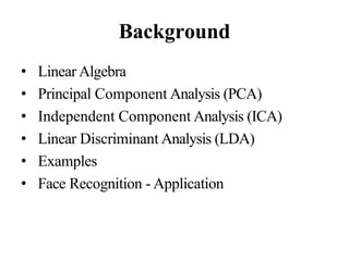
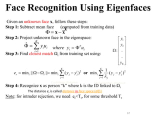
65. Suppose we are given x1, x2, ..., xM (N x 1) vectors
Step 1: compute sample mean
Step 2: subtract sample mean (i.e., center data at zero)
Step 3: compute the sample covariance matrix Σx
65
PCA - Steps
N: # of features
M: # data
1
1 M
i
i
M 
 
x x
Φi i
 
x x
i i
1 1
1 1
( )( )
M M
T T
i i
i i
M M
 
       
 
x x x x x
1 T
AA
M
where A=[Φ1 Φ2 ... ΦΜ]
i.e., the columns of A are the Φi
(N x M matrix)

66. Step 4: compute the eigenvalues/eigenvectors of Σx
Since Σx is symmetric, <u1,u2,…,uN> form an orthogonal basis in RN
and we can represent any x∈RN as:
66
PCA - Steps
1 2 ... N
  
  
1 1 2 2
1
...
N
i i N N
i
y u y u y u y u

     

x x
Note : most software packages return the eigenvalues (and corresponding eigenvectors)
is decreasing order – if not, you can explicitly put them in this order)
x i i i
u u

 
where we assume
Note : most software packages normalize ui to unit length to simplify calculations; if not, you
can explicitly normalize them)
( )
( ) || || 1
T
T
i
i i i
T
i i
u
y u if u
u u

   
x x
x x
i.e., this is
just a “change”
of basis!
1 1
2 2
. .
. .
:
. .
. .
. .
N N
x y
x y
x y
   
   
   
   
   
   
 
   
   
   
   
   
   
   
x x

67. Step 5: dimensionality reduction step – approximate x using only the
first K eigenvectors (K<<N) (i.e., corresponding to the K largest
eigenvalues where K is a parameter):
67
PCA - Steps
1 1 2 2
1
ˆ ...
K
i i K K
i
y u y u y u y u

     

x x
1 1 2 2
1
...
N
i i N N
i
y u y u y u y u

     

x x
approximate
using first K eigenvectors only
ˆ 
x x
note that if K=N, then
(i.e., zero reconstruction error)
ˆ
by
x x
1 1
2 2
1
2
. .
. .
ˆ
: : .
. .
.
. .
. . K
N N
x y
x y
y
y
y
x y
   
   
     
     
     
     
   
     
     
     
 
   
   
   
   
x x x x
(reconstruction)

68. 68
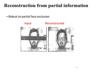
What is the Linear Transformation
implied by PCA?
• The linear transformation y = Tx which performs the
dimensionality reduction in PCA is:
1
2
ˆ
( )
.
.
T
K
y
y
U
y
 
 
 
   
 
 
 
 
x x i.e., the rows of T are the first K
eigenvectors of Σx
1
2
ˆ
( ) .
.
K
y
y
U
y
 
 
 
 
 
 
 
 
 
x x
T = UT
1 2
[ ... ] matrix
K
where U u u u N x K

i.e., the columns of U are the
the first K eigenvectors of Σx
1 1 2 2
1
ˆ ...
K
i i K K
i
y u y u y u y u

     

x x
K x N matrix

69. What is the form of Σy ?
69
i i
1 1
1 1
( )( )
M M
T T
i i
i i
M M
 
      
 
x x x x x
( )
T T
i i i
U P
   
y x x
The columns of P are the
eigenvectors of ΣX
The diagonal elements of
Λ are the eigenvalues of ΣX
or the variances
T
P P
  
x
i i
1
1
( )( )
M
T
i
M 
    

y y y y y
1
1
( )
M
T T
i i
i
P P
M 
  
 ( )
T T
P P P P
 
i i
1
1
( )( )
M
T
i
M 

 y y
1
1
( )( )
M
T T T
i i
i
P P
M 
  

1
1
( )( )
M
T T
i i
i
P P
M 
  
 T
P P
 
x

  
y
PCA de-correlates the data!
Preserves original variances!
Using diagonalization:

70. 70
Interpretation of PCA
• PCA chooses the eigenvectors of
the covariance matrix corresponding
to the largest eigenvalues.
• The eigenvalues correspond to the
variance of the data along the
eigenvector directions.
• Therefore, PCA projects the data
along the directions where the data
varies most.
• PCA preserves as much information
in the data by preserving as much
variance in the data.
u1: direction of max variance
u2: orthogonal to u1

71. Example
Compute the PCA of the following dataset:
(1,2),(3,3),(3,5),(5,4),(5,6),(6,5),(8,7),(9,8)
Compute the sample covariance matrix is:
The eigenvalues can be computed by finding the roots of the characteristic
polynomial:
71
1
1
ˆ ˆ ˆ
( )( )
n
t
k k
k
n 
   
 x μ x μ

72. Example (cont’d)
The eigenvectors are the solutions of the systems:
Note: if ui is a solution, then cui is also a solution where c≠0.
Eigenvectors can be normalized to unit-length using:
72
i i i
u u

 
x
ˆ
|| ||
i
i
i
v
v
v


73. 73
How do we choose K ?
• K is typically chosen based on how much information
(variance) we want to preserve:
• If T=0.9, for example, we “preserve” 90% of the information
(variance) in the data.
• If K=N, then we “preserve” 100% of the information in the
data (i.e., just a “change” of basis and )
1
1
( . .,0.9)
K
i
i
N
i
i
T where T is a threshold e g







ˆ 
x x
Choose the smallest
K that satisfies
the following
inequality:

74. 74
Approximation Error
• The approximation error (or reconstruction error) can be
computed by:
• It can also be shown that the approximation error can be
computed as follows:
1
1
ˆ
|| ||
2
N
i
i K

 
  
x x
ˆ
|| ||

x x
1 1 2 2
1
ˆ ...
K
i i K K
i
y u y u y u y u

      

x x x
where
(reconstruction)

75. 75
Data Normalization
• The principal components are dependent on the units used
to measure the original variables as well as on the range of
values they assume.
• Data should always be normalized prior to using PCA.
• A common normalization method is to transform all the data
to have zero mean and unit standard deviation:
i
x 

 where μ and σ are the mean and standard
deviation of the i-th feature xi

76. 76
Application to Images
• The goal is to represent images in a space of lower
dimensionality using PCA.
− Useful for various applications, e.g., face recognition, image
compression, etc.
• Given M images of size N x N, first represent each image
as a 1D vector (i.e., by stacking the rows together).
− Note that for face recognition, faces must be centered and of the
same size.

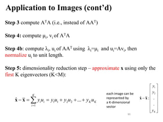
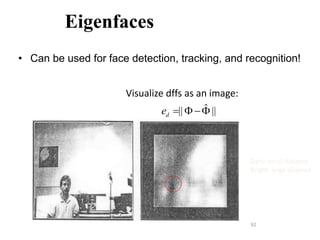
77. Application to Images (cont’d)
The key challenge is that the covariance matrix Σx is now very
large (i.e., N2 x N2) – see Step 3:
Step 3: compute the covariance matrix Σx
Σx is now an N2 x N2 matrix – computationally expensive to
compute its eigenvalues/eigenvectors λi, ui
(AAT)ui= λiui
77
1
1 1
M
T T
i
i
AA
M M

    

x i
where A=[Φ1 Φ2 ... ΦΜ]
(N2 x M matrix)

78. Application to Images (cont’d)
We will use a simple “trick” to get around this by relating the
eigenvalues/eigenvectors of AAT to those of ATA.
Let us consider the matrix ATA instead (i.e., M x M matrix)
Suppose its eigenvalues/eigenvectors are μi, vi
(ATA)vi= μivi
Multiply both sides by A:
A(ATA)vi=Aμivi or (AAT)(Avi)= μi(Avi)
Assuming (AAT)ui= λiui
λi=μi and ui=Avi
78
A=[Φ1 Φ2 ... ΦΜ]
(N2 x M matrix)

79. Application to Images (cont’d)
But do AAT and ATA have the same number of
eigenvalues/eigenvectors?
AAT can have up to N2 eigenvalues/eigenvectors.
ATA can have up to M eigenvalues/eigenvectors.
It can be shown that the M eigenvalues/eigenvectors of ATA are also the
M largest eigenvalues/eigenvectors of AAT
Steps 3-5 of PCA need to be updated as follows:
79

80. Application to Images (cont’d)
Step 3 compute ATA (i.e., instead of AAT)
Step 4: compute μi, vi of ATA
Step 4b: compute λi, ui of AAT using λi=μi and ui=Avi, then
normalize ui to unit length.
Step 5: dimensionality reduction step – approximate x using only the
first K eigenvectors (K<M):
80
1 1 2 2
1
ˆ ...
K
i i K K
i
y u y u y u y u

     

x x
each image can be
represented by
a K-dimensional
vector
1
2
ˆ : .
.
K
y
y
y
 
 
 
 

 
 
 
 
x x

81. 81
Example
Dataset

82. 82
Example (cont’d)
Top eigenvectors: u1,…uk
(visualized as an image - eigenfaces)
Mean face: x
u1
u2 u3

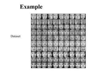
83. 83
Example (cont’d)
y=(int)255(x - fmin)/(fmax - fmin)
• How can you visualize the eigenvectors (eigenfaces) as an
image?
− Their values must be first mapped to integer values in the
interval [0, 255] (required by PGM format).
− Suppose fmin and fmax are the min/max values of a given
eigenface (could be negative).
− If xϵ[fmin, fmax] is the original value, then the new value
yϵ[0,255] can be computed as follows:

84. 84
Application to Images (cont’d)
• Interpretation: represent a face in terms of eigenfaces
1 1 2 2
1
ˆ ...
K
i i K K
i
y u y u y u y u

     

x x
x
u1 u2 u3
y1 y2 y3
1
2
ˆ : .
.
K
y
y
y
 
 
 
 

 
 
 
 
x x

85. 85
Case Study: Eigenfaces for Face Detection/Recognition
− M. Turk, A. Pentland, "Eigenfaces for Recognition", Journal of
Cognitive Neuroscience, vol. 3, no. 1, pp. 71-86, 1991.
• Face Recognition
− The simplest approach is to think of it as a template matching
problem.
− Problems arise when performing recognition in a high-dimensional
space.
− Use dimensionality reduction!

86. Process the image database (i.e., set of images with labels) –
typically referred to as “training” phase:
Compute PCA space using image database (i.e., training data)
Represent each image in the database with K coefficients Ωi
Face Recognition Using Eigenfaces
1
2
.
.
K
y
y
y
 
 
 
 
 
 
 
 
 

87. Given an unknown face x, follow these steps:
Step 1: Subtract mean face (computed from training data)
Step 2: Project unknown face in the eigenspace:
Step 3: Find closest match Ωi from training set using:
Step 4: Recognize x as person “k” where k is the ID linked to Ωi
Note: for intruder rejection, we need er<Tr, for some threshold Tr
87
Face Recognition Using Eigenfaces
2 2
1 1
1
min || || min ( ) min ( )
K K
i i
r i i i j j i j j
j j j
e y y y y

 
     
 
or
The distance er is called distance in face space (difs)
T
i i
where y u
 
1
2
: .
.
K
y
y
y
 
 
 
 

 
 
 
 
1
ˆ
K
i i
i
y u

  
  
x x
x
Euclidean distance Mahalanobis distance

88. 88
Face detection vs recognition
Detection Recognition “Sally”

89. Given an unknown image x, follow these steps:
Step 1: Subtract mean face (computed from training data):
Step 2: Project unknown face in the eigenspace:
Step 3: Compute
Step 4: if ed<Td, then x is a face.
89
Face Detection Using Eigenfaces
T
i i
where y u
 
1
ˆ
K
i i
i
y u

  
ˆ
|| ||
d
e   
x
  
x x
The ditance ed is called distance from face space (dffs)

90. 90
Eigenfaces
Reconstructed image looks
like a face.
Reconstructed image looks
like a face.
Reconstructed image
looks like a face again!
Input Reconstructed

91. 91
Reconstruction from partial information
• Robust to partial face occlusion.
Input Reconstructed

92. 92
Eigenfaces
• Can be used for face detection, tracking, and recognition!
Visualize dffs as an image:
ˆ
|| ||
d
e   
Dark: small distance
Bright: large distance

93. 93
Limitations
• Background changes cause problems
− De-emphasize the outside of the face (e.g., by multiplying the input
image by a 2D Gaussian window centered on the face).
• Light changes degrade performance
− Light normalization might help but this is a challenging issue.
• Performance decreases quickly with changes to face size
− Scale input image to multiple sizes.
− Multi-scale eigenspaces.
• Performance decreases with changes to face orientation
(but not as fast as with scale changes)
− Out-of-plane rotations are more difficult to handle.
− Multi-orientation eigenspaces.

94. 94
Limitations (cont’d)
Not robust to misalignment.

95. 95
Limitations (cont’d)
• PCA is not always an optimal dimensionality-reduction
technique for classification purposes.

96. 58
PCA Process – STEP 1
http://kybele.psych.cornell.edu/~edelman/Psych-465-Spring-2003/PCA-tutorial.pdf
0.49
1.21
0.99
0.29
1.09
0.79
 0.31
 0.81
 0.31
1.01
0.69
1.31
0.39
0.09
 1.29
0.49
0.19
 0.81
 0.31
 0.71
X '2
X1 1.81
X2 1.91
X1 X2
2.5 2.4
0.5 0.7
2.2 2.9
1.9 2.2
3.1 3.0 
2.3 2.7
2.0 1.6
1.0 1.1
1.5 1.6
1.2 0.9
X1

97. 97
PCA Process – STEP 2
• Calculate the covariance matrix
• Since the non-diagonal elements in this covariance matrix
are positive, we should expect that both the X1 and X2
variables increase together.
• Since it is symmetric, we expect the eigenvectors to be
orthogonal.
0.615444444 0.716555556
 

0.616555556 0.615444444
X
S

98. 98
PCA Process – STEP 3

0.735178656
0.677873399

 0.677873399
1.28402771 
   2 
V 
0.735178656
 
• Calculate the eigen vectors V and eigen values D
of the covariance matrix
D 
0.490833989

1 

99. PCA Process – STEP 3
Eigenvectors are plotted as
diagonal dotted lines on the
plot. (note: they are
perpendicular to each other).
One of the eigenvectors goes
through the middle of the
points, like drawing a line of
best fit.
The second eigenvector gives
us the other, less important,
pattern in the data, that all the
points follow the main line,
but are off to the side of the
main line by some amount.
99

100. 10
0
PCA Process – STEP 4
• Reduce dimensionality and form feature vector
The eigenvector with the highest eigenvalue is the principal
component of the data set.
In our example, the eigenvector with the largest eigenvalue
is the one that points down the middle of the data.
Once eigenvectors are found from the covariance matrix,
the next step is to order them by eigenvalue, highest to
lowest. This gives the components in order of significance.

101. 10
1
PCA Process – STEP 4
Now
, if you’d like, you can decide to ignorethe components
of lesser significance.
Y
ou do lose some information, but if the eigenvalues are
small, you don’t lose much
• mdimensions in your data
• calculate m eigenvectors and eigenvalues
• choose only the first r eigenvectors
• final data set has only r dimensions.

102. 10
2
PCA Process – STEP 4
• When the λi’s are sorted in descending order, the proportion
of variance explained by the r principal components is:
• If the dimensions are highly correlated, there will be a small
number of eigenvectors with large eigenvalues and r will be
much smaller than m.
• If the dimensions are not correlated, r will be as large as m
and PCA does not help.
m
p
i
r
m

i
   …  … 
   … 
 1 2
i1
i1
 1 2 r

103. 65
PCA Process – STEP 4
• Feature Vector
FeatureV
ector = (λ1 λ2 λ3 … λr)
(take the eigenvectors to keep from the ordered list of eigenvectors, and form a matrix
with these eigenvectors in the columns)
W
e can either form a feature vector with both of the
eigenvectors:
0.677873399 0.735178656
0.735178656 0.677873399 
 
or, we can choose to leave out the smaller, less significant
component and only have a single column:
0.677873399
0.735178656
 

104. 10
4
PCA Process – STEP 5
• Derive the new data
FinalData = RowFeatureVector x RowZeroMeanData
RowFeatureVector is the matrix with the
eigenvectors in the columns transposed so that the
eigenvectors are now in the rows, with the most
significant eigenvector at the top.
RowZeroMeanData is the mean-adjusted data
transposed, i.e., the data items are in each column,
with each row holding a separate dimension.

105. 10
5
PCA Process – STEP 5
• FinalData is the final data set, with data items in
columns, and dimensions along rows.
• What does this give us?
The original data solely in terms of the vectors
we chose.
• We have changed our data from being in terms
of the axes X1 and X2, to now be in terms of
our 2 eigenvectors.

106. 10
6
PCA Process – STEP 5
FinalData (transpose: dimensions along columns)
Y2
 0.175115307
0.142857227
0.384374989
0.130417207
 0.209498461
0.175282444
 0.349824698
0.0464172582
0.0177646297
 0.162675287
Y1
 0.827870186
1.77758033
 0.992197494
 0.274210416
1.67580142
 0.912949103
0.0991094375
1.14457216
0.438046137
1.22382956

107. PCA Process – STEP 5
10
7

108. 10
8
Reconstruction of Original Data
• Recall that:
FinalData = RowFeatureVector x RowZeroMeanData
• Then:
RowZeroMeanData = RowFeatureVector-1 x FinalData
• And thus:
RowOriginalData = (RowFeatureVector-1 x FinalData) +
OriginalMean
• If we use unit eigenvectors, the inverse is the same
as the transpose (hence, easier).

109. 10
9
Reconstruction of Original Data
• If we reduce the dimensionality (i.e., r < m),
obviously, when reconstructing the data we lose
those dimensions we chose to discard.
• In our example let us assume that we considered
only a single eigenvector.
• The final data is Y1 only and the reconstruction
yields…

110. Reconstruction of Original Data
The variation along
the principal
component is
preserved.
The variation along
the other component
has been lost.
11
0

111. References
• J. SHLENS, "TUTORIAL ON PRINCIPAL
COMPONENT ANALYSIS," 2005
http://www.snl.salk.edu/~shlens/pub/notes/pca.pdf
• Introduction to PCA,
http://dml.cs.byu.edu/~cgc/docs/dm/Slides/