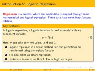
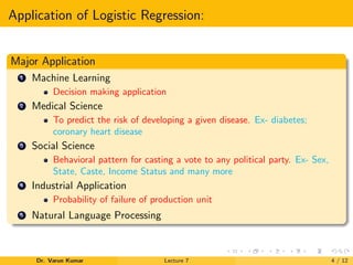
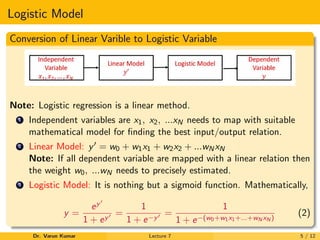
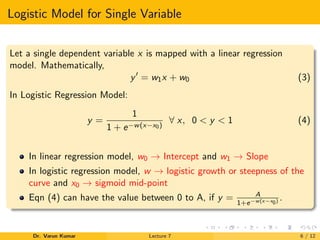
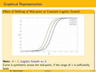
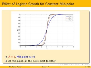
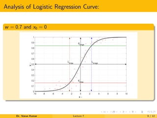
This document provides an introduction to logistic regression. It outlines key features such as using a logistic function to model a binary dependent variable that can take on values of 0 or 1. Logistic regression is a linear method that uses the logistic function to transform predictions. The document discusses applications in machine learning, medical science, social science, and industry. It also provides details on logistic regression models, including converting linear variables to logistic variables using a sigmoid function and examining the effects of varying the logistic growth and midpoint parameters on the logistic regression curve.

1. Logistic Regression
Dr. Varun Kumar
Dr. Varun Kumar Lecture 7 1 / 12

2. Outlines
1 Introduction to Logistic Regression
2 Linear vs Logistic Regression
3 Sigmoid Function
4 References
Dr. Varun Kumar Lecture 7 2 / 12

3. Introduction to Logistic Regression:
Regression is a process, where real world data is mapped through some
mathematical and logical expression. These data have some input/output
relation.
Key Features
In logistic regression, a logistic function is used to model a binary
dependent variable.
y = f (x) (1)
Here, y can take only two value, i.e 0 and 1.
1 Logistic regression is a linear method, but the predictions are
transformed using the logistic function.
2 It is also called as binary regression.
3 Decision is taken either 0 or 1, low or high, no or yes.
Dr. Varun Kumar Lecture 7 3 / 12

4. Application of Logistic Regression:
Major Application
1 Machine Learning
Decision making application
2 Medical Science
To predict the risk of developing a given disease. Ex- diabetes;
coronary heart disease
3 Social Science
Behavioral pattern for casting a vote to any political party. Ex- Sex,
State, Caste, Income Status and many more
4 Industrial Application
Probability of failure of production unit
5 Natural Language Processing
Dr. Varun Kumar Lecture 7 4 / 12

5. Logistic Model
Conversion of Linear Varible to Logistic Variable
Note: Logistic regression is a linear method.
1 Independent variables are x1, x2, ...xN needs to map with suitable
mathematical model for finding the best input/output relation.
2 Linear Model: y = w0 + w1x1 + w2x2 + ...wNxN
Note: If all dependent variable are mapped with a linear relation then
the weight w0, ...wN needs to precisely estimated.
3 Logistic Model: It is nothing but a sigmoid function. Mathematically,
y =
ey
1 + ey
=
1
1 + e−y
=
1
1 + e−(w0+w1x1+...+wN xN )
(2)
Dr. Varun Kumar Lecture 7 5 / 12

6. Logistic Model for Single Variable
Let a single dependent variable x is mapped with a linear regression
model. Mathematically,
y = w1x + w0 (3)
In Logistic Regression Model:
y =
1
1 + e−w(x−x0)
∀ x, 0 < y < 1 (4)
In linear regression model, w0 → Intercept and w1 → Slope
In logistic regression model, w → logistic growth or steepness of the
curve and x0 → sigmoid mid-point
Eqn (4) can have the value between 0 to A, if y = A
1+e−w(x−x0) .
Dr. Varun Kumar Lecture 7 6 / 12

7. Graphical Representation
Effect of Shifting of Mid-point at Constant Logistic Growth
-10 -8 -6 -4 -2 0 2 4 6 8 10
x→
0
0.1
0.2
0.3
0.4
0.5
0.6
0.7
0.8
0.9
1
y→
w=1,x0
=0
w=1,x0
=-1
w=1,x0
=1
Note: A = 1, Logistic Growth w=1
Curve is symmetric across the mid-point, if the range of x is sufficiently
large.
Dr. Varun Kumar Lecture 7 7 / 12

8. Effect of Logistic Growth for Constant Mid-point
-10 -8 -6 -4 -2 0 2 4 6 8 10
x→
0
0.1
0.2
0.3
0.4
0.5
0.6
0.7
0.8
0.9
1
y→
w=1, x0
=0
w=2, x0
=0
w=3, x0
=0
A = 1, Mid-point x0=0
At mid-point, all the curve meet together.
Dr. Varun Kumar Lecture 7 8 / 12

9. Analysis of Logistic Regression Curve:
w = 0.7 and x0 = 0
-10 -8 -6 -4 -2 0 2 4 6 8 10
x→
0
0.1
0.2
0.3
0.4
0.5
0.6
0.7
0.8
0.9
1
y→
*
*
*
*
* ** *
*
*
*
**
*
*
*
*
*
*
* *
*
*
*
*
*
*
*
*
*
*
*
*
*
*
*
LH-low
LH-high
dV-low
dV-high
Dr. Varun Kumar Lecture 7 9 / 12

10. Continued–
In above curve, logistic function lies between -10 to 10.
Above curve is showing symmetry across 0, where the value logistic
expression is 0.5.
Higher the logistic growth w greater be accuracy for taking the
decision, either in favor of 0 or 1.
Lower the logistic growth w, the decision accuracy decreases with
significant proportion.
Most of the practical system does not have a very high value of
logistic growth parameter w.
50% decision threshold is not showing a precise devise.
Estimation of w and x0 is relatively more difficult compare to linear
regression weight coefficient w1 and w0.
Dr. Varun Kumar Lecture 7 10 / 12

11. Continued–
Let 0.9 < y < 1 → Decision in favor 1 is a good machine compare to
0.5 < y < 1 → Decision in favor 1.
Similarly, 0 < y < 0.1 → Decision in favor 0 is a good machine
compare to 0 < y < 0.5 → Decision in favor 0.
From Figure 3, higher the value (dV −high − dV −low ) greater be the
quality machine or system.
From Figure 3, the data point for having logistic expression lies
between dV −low < y < dV −high is not acceptable. In another sense
LH−low < x < LH−high is not acceptable that causes error for making
a good machine.
Dr. Varun Kumar Lecture 7 11 / 12

12. References
E. Alpaydin, Introduction to machine learning. MIT press, 2020.
J. Grus, Data science from scratch: first principles with python. O’Reilly Media,
2019.
T. M. Mitchell, The discipline of machine learning. Carnegie Mellon University,
School of Computer Science, Machine Learning , 2006, vol. 9.
Dr. Varun Kumar Lecture 7 12 / 12