Downloaded 224 times

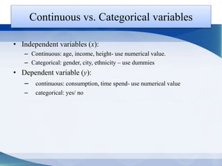
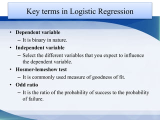
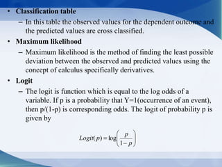

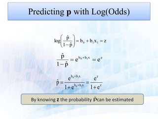
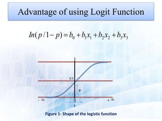
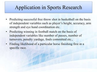
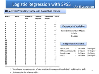
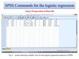
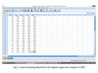
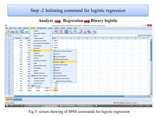
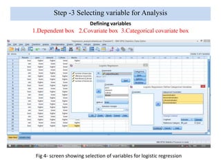
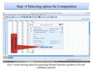
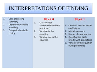
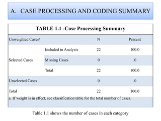
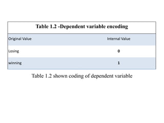
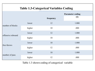
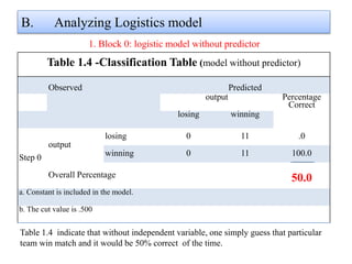
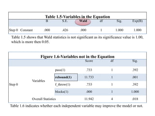
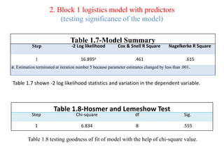
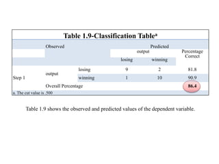
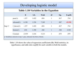
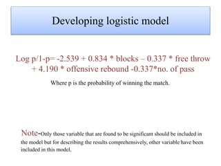
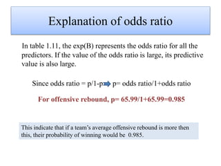
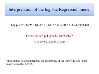


Logistic regression is used to predict categorical outcomes. The presented document discusses logistic regression, including its objectives, assumptions, key terms, and an example application to predicting basketball match outcomes. Logistic regression uses maximum likelihood estimation to model the relationship between a binary dependent variable and independent variables. The document provides an illustrated example of conducting logistic regression in SPSS to predict match results based on variables like passes, rebounds, free throws, and blocks.


![제 23회 보아즈(BOAZ) 빅데이터 컨퍼런스 - [MBOAX] : ABSA를 활용한 소비자 반응 분석 기반 운영 효율화 대시보드 설계](https://cdn.slidesharecdn.com/ss_thumbnails/3-1boaz23rdconferencemboax-260203102709-9d519923-thumbnail.jpg?width=640&height=640&fit=bounds)