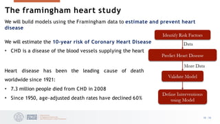
The document outlines a lesson on logistic regression, focusing on its use for classification problems where response variables are categorical rather than continuous. It explains why linear regression is inadequate for such cases and details the formulation of logistic regression, including its cost function and application to various classification scenarios. Additionally, it introduces the Framingham Heart Study as a case study for applying logistic regression to estimate the risk of coronary heart disease.

1. Lesson
3.
Logistic regression
TEACHER
Antonio Ferramosca
PLACE
University of Bergamo
DYNAMIC SYSTEMS
IDENTIFICATION COURSE
MASTER DEGREE
ENGINEERING AND
MANAGEMENT FOR HEALTH

2. Outline
2 /33
1. The classification problem
2. Why not linear regression?
3. Logistic regression formulation
4. Logistic regression cost function
5. Worked examples

3. Outline
3 /33
1. The classification problem
2. Why not linear regression?
3. Logistic regression formulation
4. Logistic regression cost function
5. Worked examples

4. The linear regression model discussed in the previous lesson assumes that
the response variable 𝑦 is quantitative (metrical)
• in many situations, the response variable is instead qualitative (categorical)
Qualitative variables take values in an unordered set 𝒞 = "cat1", … , "catC" , such as:
• eye color ∈ "brown", "blue", "green"
• email ∈ "spam", "not spam"
4 /33
Metric data
• Describe a quantity
• An ordering is defined
• A distance is defined
Categorical data
• Describe membership categories
• It is not meaningful to apply an ordering
• It is not meaningful to compute
distances
The classification
probelm

5. The process of estimating categorical outcomes using a set of regressors 𝝋 is called
classification
Estimating a categorical response for an observation 𝝋 can be referred to as
classifying that observation, since it involves assigning the observation to a
category, or class
Often we are more interested in estimating the probabilities that 𝝋 belongs to
each category in 𝒞
The most probable category is then chosen as the class for the observation 𝝋
5 /33
The classification probelm

6. Examples of classification
problems
6 /33
• A person arrives at the emergency room with a set of symptoms that could possibly
be attributed to one of three medical conditions
Which of the three conditions does the individual have?
• Anonline banking system manages transactions, storing user’s IP address,
past transaction history, and so forth
Is the transaction fraudulent or not?
• A biologist collects DNA sequence data for a number of patients with and without
a given disease
which DNA mutations are deleterious (disease-causing) and which are not?

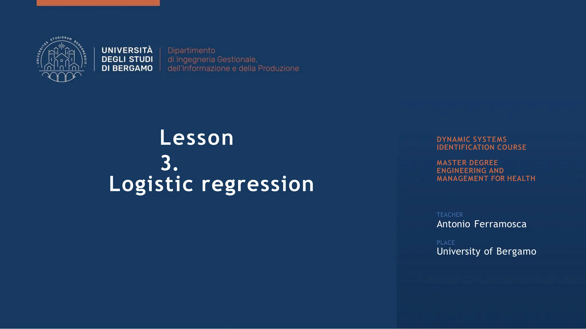
7. Example: cat vs dog classification
𝜑1 Weight [kg]
Height
[cm]
Cats
Dogs
Classifier function 𝑓
⋅
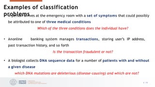
Suppose that we measure the weight and
height of some dogs and cats
We want to learn the function 𝑓 ⋅ that
can tell us if a given input vector 𝝋 = 𝜑1,
𝜑2
𝖳 is a dog or a cat
• 𝜑1: weight
• 𝜑2: height
QUIZ: The point is classified by the model
as a ?
𝜑2
7 /33

8. The classification
problem
QUIZ: Consider a company that produces sliding gates. The gates can have four
weights 300Kg, 400Kg, 500Kg, 600Kg . We want to detect the weight
of the gate. This is a:
 A regression problem
 A classification problem
 Both a regression and a classification problem
8 /33

9. Outline
9 /33
1. The classification problem
2. Why not linear
regression?
3. Logistic regression formulation
4. Logistic regression cost function
5. Worked examples

10. Why not linear regression?
10 /33
Suppose that we are trying to estimate the medical condition of a patient in the
emergency room based on her symptoms
There are three possibilities: stroke, drug overdose and epileptic seizure
We could consider encoding these values as a quantitative response variable, 𝑦, as
1 if stroke
𝑦 = <2 if drug overdose
3 if epileptic
seizure
However, we are implicitly saying that the «difference» between drug overdose and
stroke is the same as the «difference» between epileptic seizure and drug
overdose, which does not make much sense

11. Why not linear regression?
11 /33
We can also change the encoding to
1 if epileptic seizure
𝑦 = <2 if stroke
3 if drug overdose
This would imply a totally different relationship among the three conditions
• each of these codings would produce fundamentally different linear models…
• …that would ultimately lead to different sets of estimates on test observations
In general, there is no natural way to convert a qualitative response variable with more
than two levels into a quantitative response that is ready for linear regression

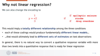
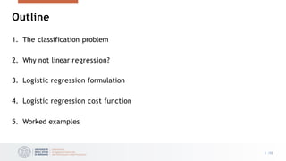
12. Why not linear regression?
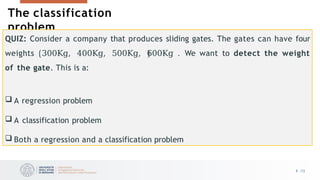
With two levels, the situation is better. For instance, perhaps there are only two
possibilities for the patient’s medical condition: stroke and drug overdose
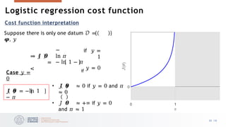
0 if
stroke
𝑦 = <
1
if
drug overdose
We can fit a linear regression to this binary response, and classify as drug overdose if
𝑦C > 0.5 and stroke otherwise, interpreting 𝑦C as a probability of drug overdose
However, if we use linear regression, some of our estimates might be outside the [0, 1]
interval, which does not make sense as a probability. There is nothing that “saturates” the
output between 0 and 1. Logistic function (Sigmoid)
12 /33

13. Outline
13 /33
1. The classification problem
2. Why not linear regression?
3. Logistic regression formulation
4. Logistic regression cost function
5. Worked examples

14. Logistic regression
Purpose: Estimate the probability that a set of input regressors 𝝋 ∈ ℝ𝑑×1 belong to
one of two classes 𝑦 ∈ 0, 1
Logistic function (Sigmoid)
Define the linear combination quantity
𝑑–1
𝑎 = I 𝜑𝑖 ⋅ 𝜃𝑖 = 𝝋𝖳 ⋅
𝜽
𝑖=0
The formula 𝑠 𝑎 is the logistic function
𝑠
𝑎
1 𝑒𝑎
=
1 + 𝑒– 𝑎 =
1
+ 𝑒𝑎
• 𝑎 ≫ 0 ⇒ 𝑠 𝑎
= 1
• 𝑎 ≪ 0 ⇒ 𝑠 𝑎
= 0
0.
5
14 /33
0

15. Logistic regression
Purpose: Estimate the probability that a set of input regressors 𝝋 ∈ ℝ𝑑×1 belong to
one of two classes 𝑦 ∈ 0, 1
𝑃 𝑦 = 1 𝝋 = 𝑠 𝑎
= 𝑠 𝝋𝖳𝜽 =
1
1 + 𝑒–
𝝋𝖳 𝜽
• 𝝋𝖳𝜽 ≪ 0 ⇒ 𝑠 𝝋𝖳𝜽≪ 0.5 ⇒ 𝑃 𝑦 =
1 𝝋 ≈ 0
The output of 𝑠 𝝋𝖳𝜽 is interpreted as a probability
• 𝝋𝖳𝜽 ≫ 0 ⇒ 𝑠 𝝋𝖳𝜽 ≫ 0.5 ⇒ 𝑃 𝑦 = 1 𝝋 ≈ 1 𝝋 is
classified to class 1
𝝋 is classified to class
0
15 /33

16. Outline
16 /33
1. The classification problem
2. Why not linear regression?
3. Logistic regression formulation
4. Logistic regression cost
function
5. Worked examples

17. Logistic regression cost function
where
𝝋 𝑖
∈
ℝ𝑑×1
Suppose to have at disposal a dataset 𝒟 = 𝝋 1 , 𝑦 1 , … ,
𝝋 𝑁 , 𝑦 𝑁
and 𝑦 𝑖 ∈ 0, 1 , 𝑖 = 1, … , 𝑁, 𝑖. 𝑖. 𝑑.
Estimate a logistic regression model 𝑃 𝑦
𝑖
= 1 𝝋 𝑖
=
1
1 + 𝑒–𝝋 𝑖
𝖳 𝜽
≡
𝜋 𝑖
𝑁
𝐽𝜽 = − 7 𝑦 𝑖 ⋅ ln 𝜋 𝑖 +
1 − 𝑦 𝑖
𝑖=1
⋅ ln 1
− 𝜋
𝑖
The logistic regression cost function 𝐽 𝜽 is
defined as:
17 /33

18.  In the ln terms
 In the 𝜋 𝑖
terms
QUIZ: In the logistic regression cost function, where are the parameters 𝜽 that
we want to estimate?
𝑁
𝐽 𝜽 = − 7 𝑦 𝑖
⋅ ln 𝜋 𝑖
+ 1 − 𝑦 𝑖
𝑖=1
 In the 𝑦 𝑖 terms
⋅ ln 1
− 𝜋
𝑖
18 /33
Logistic regression cost function

19. Logistic regression cost function
Cost function interpretation
Suppose there is only one datum 𝒟 =
𝝋, 𝑦
⇒ 𝐽 𝜽
=
<
−
ln 𝜋
− ln 1 − 𝜋
if
if 𝑦 =
1
𝑦 = 0
Case 𝑦 =
1
𝐽 𝜽 =
−ln 𝜋
• 𝐽 𝜽 ≈ 0 if 𝑦 = 1 and 𝜋
≈ 1
• 𝐽 𝜽 ≈ +∞ if 𝑦 = 1
and 𝜋 ≈ 0
19 /33

20. Logistic regression cost function
Cost function interpretation
Suppose there is only one datum 𝒟 =
𝝋, 𝑦
⇒ 𝐽 𝜽
=
<
−
ln 𝜋
− ln 1 − 𝜋
if
if 𝑦 =
1
𝑦 = 0
Case 𝑦 =
0
𝐽 𝜽 = −ln 1
− 𝜋
• 𝐽 𝜽 ≈ 0 if 𝑦 = 0 and 𝜋
≈ 0
• 𝐽 𝜽 ≈ +∞ if 𝑦 = 0
and 𝜋 ≈ 1
20 /33

21. We have to compute the gradient of 𝐽 𝜽 with respect to 𝜽 ∈ ℝ𝑑×1. First, compute
the
derivative of 𝑠 𝑎
=
1
1+𝑒"
𝑎
𝜕𝑠 𝑎
=
𝜕 1
𝜕
𝜕𝑎 𝜕𝑎 1 + 𝑒"𝑎 =
𝜕
𝑎
1 + 𝑒"𝑎 "1 =
= 1
𝑒"𝑎
1 + 𝑒"𝑎 ⋅
1 +
𝑒"𝑎
= ⋅
1 1 + 𝑒"𝑎
− 1
1 + 𝑒"𝑎 1 + 𝑒"𝑎
1 1 + 𝑒"𝑎
1
=
1 + 𝑒"𝑎 ⋅
1 + 𝑒"𝑎 −
1 +
𝑒"𝑎
=
𝝋 ⋅ 𝜋 ⋅ 1
− 𝜋
In the case where 𝑎 = 𝝋𝖳𝜽, we have that
𝛻𝜽𝑠 𝝋𝖳𝜽 = 𝝋 ⋅ 𝑠
𝝋𝖳𝜽 ⋅ 1 − 𝑠 𝝋𝖳𝜽 =
𝑑×1 𝑑×1 1×1
1×1
− 1
+ 𝑒
"𝑎 "2 "𝑎
𝑒 −1 = − 1 +
𝑒
"𝑎 "2 "𝑎
−𝑒
=
𝑒"𝑎
1 + 𝑒"𝑎
2
𝑠 𝑎 ⋅ 1 − 𝑠 𝑎
21 /33
IN-DEPTH ANALYSIS
Computation of the minimum of
𝐽(𝜽)

22. We can now compute the gradient of
𝐽 𝜽
𝑁
𝐽
𝜽
= − 3 𝑦 𝑖 ln 𝜋 𝑖 + 1 − 𝑦 𝑖
ln 1 − 𝜋 𝑖
𝑖=1
𝜋
𝑖
1
=
1 + 𝑒−𝝋 𝑖
𝑇𝜽
𝑁
𝛻𝜽𝐽 𝜽=
− /
𝑑×1
𝑖=1
𝑦
𝑖
𝜋
′ 𝑖
𝜋
𝑖
+ 1 − 𝑦
𝑖
−𝜋
′ 𝑖
1 − 𝜋
𝑖
𝑁
= − /
𝑦 𝑖
𝑖=1
𝝋 𝑖 𝜋
𝑖
1 − 𝜋
𝑖
𝜋
𝑖
+ 1 − 𝑦
𝑖
−𝝋 𝑖 𝜋 𝑖 1
− 𝜋 𝑖 1
− 𝜋 𝑖
1 − 𝜋
𝑖
− 1 − 𝑦
𝑖
−𝝋 𝑖 𝜋
𝑖
𝑁
= / −𝑦 𝑖 𝝋
𝑖
𝑖=1
𝑁
𝑁
= / 𝝋 𝑖 ⋅ −𝑦 𝑖 + 𝑦
𝑖 𝜋 𝑖
𝑖=1
+ 𝝋 𝑖 ⋅ 𝜋 𝑖 − 𝑦
𝑖 𝜋 𝑖
= / 𝝋 𝑖 ⋅ −𝑦 𝑖 + 𝑦 𝑖 𝜋 𝑖 −
𝑦 𝑖 𝜋 𝑖 + 𝜋 𝑖
𝑖=1
𝑖=
1
𝑁
= / 𝝋 𝑖⋅ 𝜋 𝑖 −
𝑦 𝑖
𝑑×1 1×1
IN-DEPTH ANALYSIS
Computation of the minimum of
𝐽(𝜽)
22 /33

23. It can be shown that:
• The cost function 𝐽 𝜽 is convex and admits a unique minimum
• The equations found by posing 𝛻𝜽𝐽 𝜽 = 𝟎 are nonlinear in 𝜽 and it is not
possible to find a solution in closed-form
 For this reason, we need to resort to iterative optimization algorithms
Use gradient descent:
𝜽 9 𝜽:
𝑘
𝜽! 𝑘 + 1 = 𝜽! 𝑘
− 𝛼 ⋅ 𝛻𝐽 𝜽 ,
𝑑×1 𝑑×1 1×1 𝑑×1
𝛼 ∈ ℝ/0: learning
rate
Gradient descent
23 /33

24. Gradient descent
⋅ −𝜑1
𝑖
𝑁
𝜃0 = 𝜃0 − 𝛼 ⋅ I 𝜋 𝑖
−
𝑦 𝑖
𝑖=1
𝑁
𝜃1 = 𝜃2 − 𝛼 ⋅ I 𝜋 𝑖
−
𝑦 𝑖
𝑖=1
Repeat {
�
�
𝜃𝑑–1 = 𝜃𝑑–1 − 𝛼 ⋅ I 𝜋 𝑖 −
𝑦 𝑖
𝑖=1
⋅ −𝜑𝑑–1
𝑖
⋮
}
𝑁
𝐽𝜽 = − 7 𝑦 𝑖 ⋅ ln 𝜋 𝑖 +
1 − 𝑦 𝑖
𝑖=1
⋅ ln 1
− 𝜋
𝑖
24 /33

25. The logistic regression model, despite its name, is not used for regression, but for
classification
Once the model estimates the probability of a class, we can classify a point to a particular
class if the probability for that class is above a threshold (usually 0.5)
The function that now we are trying to estimate is: 𝑓 𝝋 = 𝑃 𝑦 = 1 𝝋
The logistic regression tries to model 𝑓 by using the model:
𝑠 𝝋𝖳𝜽
=
1
1 + 𝑒–
𝝋𝖳 𝜽
The point 𝝋 can then be classified to class 𝑦 = +1 if 𝑠
𝝋𝖳𝜽 ≥ 0.5
25 /33
Logistic regression recap

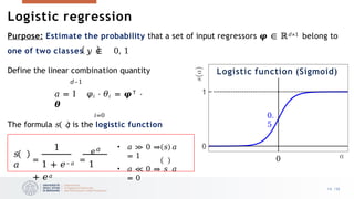
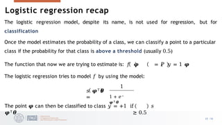
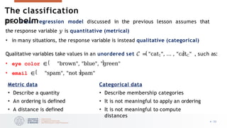
26. Logistic regression recap
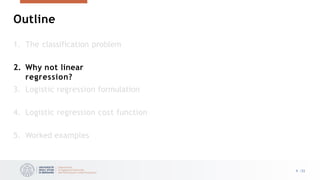
The classification boundary found by
logistic regression is linear
Infact, classifying with the rule:
𝑦 = 1 if 𝑠 𝝋𝖳𝜽 ≥ 0.5
is the same as saying
𝑦 = 1 if 𝝋𝖳𝜽 ≥ 0
Weight [kg]
Height
[cm]
Cats
Dogs
Linear classifier
26 /33

27. Outline
27 /33
1. The classification problem
2. Why not linear regression?
3. Logistic regression formulation
4. Logistic regression cost function
5. Worked examples

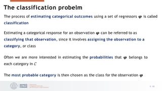
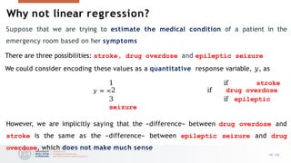
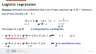
28. We want to estimate if a student will get admitted
to a university given the results on two exams (𝜑1, 𝜑2)
• The training set consists of 𝑁 = 100 students
with
𝜑1 𝑖 , 𝜑2 𝑖 and 𝑦 𝑖 ∈ 0,1 , for 𝑖 = 1, … , 𝑁
•
•
•
Φ ∈
ℝ100×3
𝒚 ∈
ℝ100×1
𝜽 ∈ ℝ3×1
% Read data from file
data = load(‘studentsdata.csv’);
Phi = data(:, [1, 2]); y = data(:, 3);
% Setup the data matrix appropriately, and
add ones for the intercept term
[N, m] = size(Phi); d = m + 1;
% Add intercept term
Phi = [ones(N, 1) Phi];
% Initialize fitting parameters
initial_theta = zeros(d, 1);
pi_s = sigmoid(Phi*theta)
J = ( -y'*log(pi_s) – (1-y)'*log(1-pi_s));
grad = Phi'*( pi_s - y);
Embed in a function and pass the function to an
optimization algoritm that iteratively computes
the gradient
28 /33
Students admissions classification

29. The framingham heart study
29 /33
In late 1940s, U.S. Government set out to better understand cardiovascular disease
Plan: track large cohort of initially healthy patients over time
The city of Framingham (MA) was selected as site for the study in the 1948
• Appropriate size
• Stable population
• Cooperative doctors and residents
A total of 5209 patients aged 30-59 were enrolled. They had to give a survey and take
and exam every 2 years:
• Physical characteristics and behavioral characteristics
• Test results

30. The framingham heart study
We will build models using the Framingham data to estimate and prevent heart
disease
We will estimate the 10-year risk of Coronary Heart Disease
• CHD is a disease of the blood vessels supplying the heart
Heart disease has been the leading cause of death
worldwide since 1921:
• 7.3 million people died from CHD in 2008
• Since 1950, age-adjusted death rates have declined 60%
30 /33

31. The framingham heart study
31 /33
Demographic risk factors
• male: sex of patient
• education: Some high school (1), high school (2), some college (3), college
(4)
Behavioral risk factors
• currentSmoker: 0/1
Behavioral risk factors
• BPmeds: On blood pressure medication at time of first examination
• prevalentStroke: Previously had a stroke
• prevalentHyp: Currently hypertensive
• cigsPerDay: cigarettes per day
• age: age in years at first examination
• Diabetes: Currently has diabetes

32. The framingham heart study
32 /33
Risk factors from first examination
• totChol: Total cholesterol (mg/dL)
• sysBP: Systolic blood pressure
• diaBP: Diastolic blood pressure
• BMI: Body Mass Index (kg/m2)
• heartRate: Heart rate (beats/minute)
• glucose: Blood glucose level (mg/dL)
Use logistic regression to estimate whether or not a patient experienced CHD within
10 years of first examination

33. The framingham heart
study
Most critical identified risk
factors
33 /33

34. UNIVE RSITA
DEGLI STUDI
DI BERGAMO