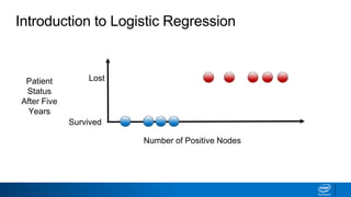
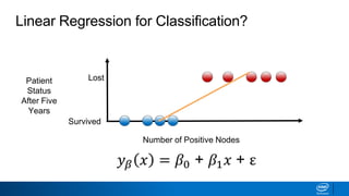
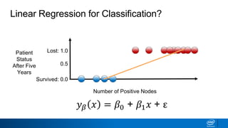
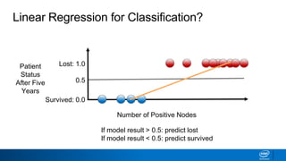
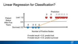
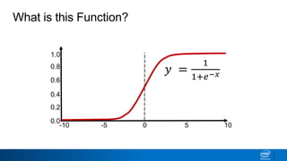
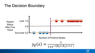
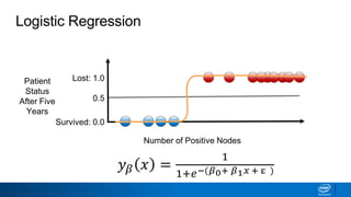
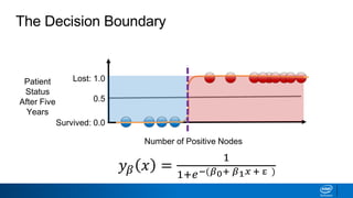
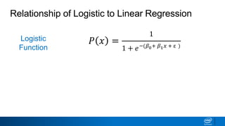
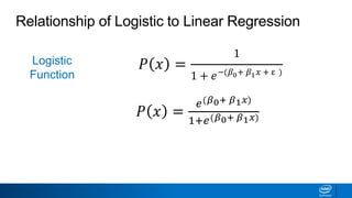
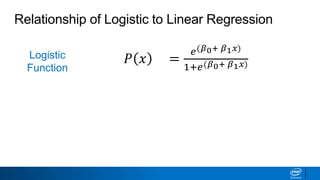
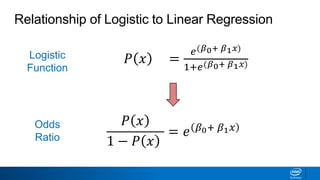
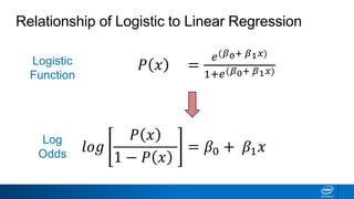
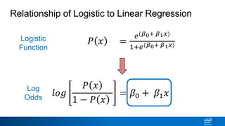
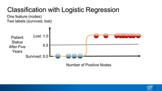
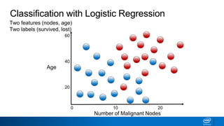
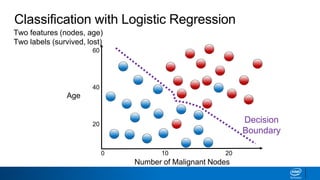
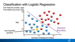
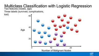
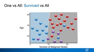
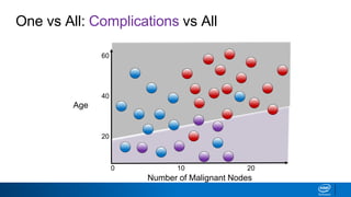
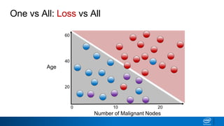
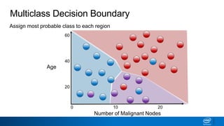
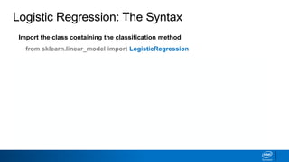
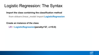
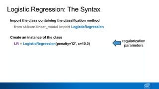
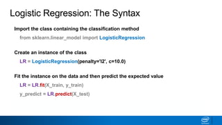
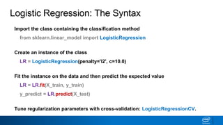
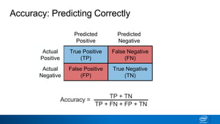
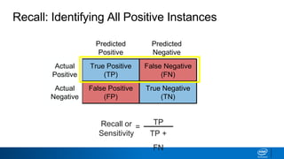
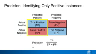
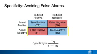
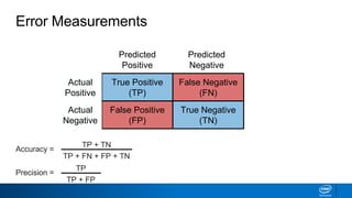
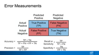
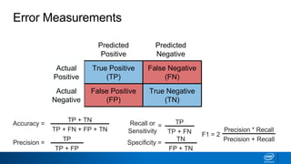
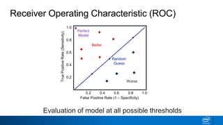
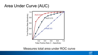
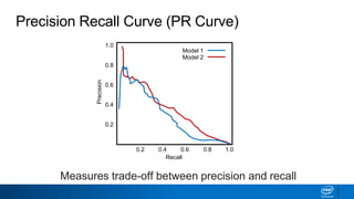
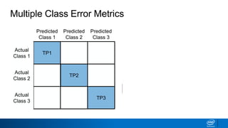
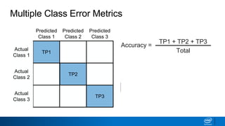
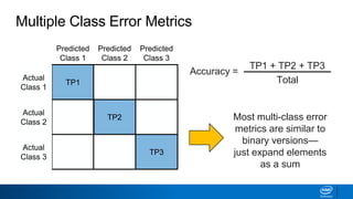
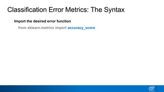
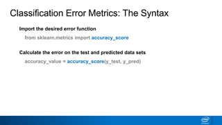
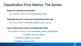
This document provides an introduction to logistic regression. It begins by explaining how linear regression is not suitable for classification problems and introduces the logistic function which maps linear regression output between 0 and 1. This probability value can then be used for classification by setting a threshold of 0.5. The logistic function models the odds ratio as a linear function, allowing logistic regression to be used for binary classification. It can also be extended to multiclass classification problems. The document demonstrates how logistic regression finds a decision boundary to separate classes and how its syntax works in scikit-learn using common error metrics to evaluate performance.

1. Logistic Regression

2. Legal Notices and Disclaimers
This presentation is for informational purposes only. INTEL MAKES NO WARRANTIES,
EXPRESS OR IMPLIED, IN THIS SUMMARY.
Intel technologies’ features and benefits depend on system configuration and may require
enabled hardware, software or service activation. Performance varies depending on system
configuration. Check with your system manufacturer or retailer or learn more at intel.com.
This sample source code is released under the Intel Sample Source Code License Agreement.
Intel and the Intel logo are trademarks of Intel Corporation in the U.S. and/or other countries.
*Other names and brands may be claimed as the property of others.
Copyright © 2017, Intel Corporation. All rights reserved.

3. Introduction to Logistic Regression
Number of Positive Nodes
Patient
Status
After Five
Years
Survived
Lost

4. Linear Regression for Classification?
Number of Positive Nodes
Survived
LostPatient
Status
After Five
Years
𝑦 𝛽 𝑥 = 𝛽0 + 𝛽1 𝑥 + ε

5. Linear Regression for Classification?
Number of Positive Nodes
Survived: 0.0
Lost: 1.0Patient
Status
After Five
Years
0.5
𝑦 𝛽 𝑥 = 𝛽0 + 𝛽1 𝑥 + ε

6. Linear Regression for Classification?
Number of Positive Nodes
Survived: 0.0
Lost: 1.0Patient
Status
After Five
Years
If model result > 0.5: predict lost
If model result < 0.5: predict survived
0.5

7. Linear Regression for Classification?
Number of Positive Nodes
Survived: 0.0
Lost: 1.0Patient
Status
After Five
Years
If model result > 0.5: predict lost
If model result < 0.5: predict survived
0.5
0 0
0000
1 1 1 1 1 1 1
Prediction

8. What is this Function?
0.0
1.0
0.2
0.4
0.6
0.8
0-5-10 5 10
𝑦 =
1
1+𝑒−𝑥

9. The Decision Boundary
Number of Positive Nodes
Survived: 0.0
Lost: 1.0Patient
Status
After Five
Years
0.5
𝑦 𝛽 𝑥 =
1
1+𝑒−(𝛽0+ 𝛽1 𝑥 + ε )

10. Logistic Regression
Number of Positive Nodes
Survived: 0.0
Lost: 1.0Patient
Status
After Five
Years
0.5
𝑦 𝛽 𝑥 =
1
1+𝑒−(𝛽0+ 𝛽1 𝑥 + ε )

11. The Decision Boundary
Number of Positive Nodes
Survived: 0.0
Lost: 1.0Patient
Status
After Five
Years
0.5
𝑦 𝛽 𝑥 =
1
1+𝑒−(𝛽0+ 𝛽1 𝑥 + ε )

12. Relationship of Logistic to Linear Regression
Logistic
Function
𝑃 𝑥 =
1
1 + 𝑒−(𝛽0+ 𝛽1 𝑥 + ε )

13. Relationship of Logistic to Linear Regression
Logistic
Function
𝑃 𝑥 =
1
1 + 𝑒−(𝛽0+ 𝛽1 𝑥 + ε )
𝑃 𝑥 =
𝑒(𝛽0+ 𝛽1 𝑥)
1+𝑒(𝛽0+ 𝛽1 𝑥)

14. Relationship of Logistic to Linear Regression
Logistic
Function
𝑃 𝑥 =
𝑒(𝛽0+ 𝛽1 𝑥)
1+𝑒(𝛽0+ 𝛽1 𝑥)

15. Relationship of Logistic to Linear Regression
𝑃 𝑥 =
𝑒(𝛽0+ 𝛽1 𝑥)
1+𝑒(𝛽0+ 𝛽1 𝑥)
𝑃 𝑥
1 − 𝑃 𝑥
= 𝑒 𝛽0+ 𝛽1 𝑥
Logistic
Function
Odds
Ratio

16. 𝑙𝑜𝑔
𝑃 𝑥
1 − 𝑃 𝑥
= 𝛽0 + 𝛽1 𝑥
Relationship of Logistic to Linear Regression
𝑃 𝑥 =
𝑒(𝛽0+ 𝛽1 𝑥)
1+𝑒(𝛽0+ 𝛽1 𝑥)
Logistic
Function
Log
Odds

17. 𝑙𝑜𝑔
𝑃 𝑥
1 − 𝑃 𝑥
= 𝛽0 + 𝛽1 𝑥
Relationship of Logistic to Linear Regression
𝑃 𝑥 =
𝑒(𝛽0+ 𝛽1 𝑥)
1+𝑒(𝛽0+ 𝛽1 𝑥)
Logistic
Function
Log
Odds

18. Classification with Logistic Regression
Number of Positive Nodes
Survived: 0.0
Lost: 1.0Patient
Status
After Five
Years
0.5
One feature (nodes)
Two labels (survived, lost)

19. Number of Malignant Nodes
0
Age
60
40
20
10 20
Two features (nodes, age)
Two labels (survived, lost)
Classification with Logistic Regression

20. Number of Malignant Nodes
0
Age
60
40
20
10 20
Two features (nodes, age)
Two labels (survived, lost)
Classification with Logistic Regression
Decision
Boundary

21. Number of Malignant Nodes
0
Age
60
40
20
10 20
Two features (nodes, age)
Two labels (survived, lost)
new example
(predict)
Classification with Logistic Regression
Decision
Boundary

22. Number of Malignant Nodes
0
Age
60
40
20
10 20
Two features (nodes, age)
Three labels (survived, complications,
lost)
Multiclass Classification with Logistic Regression

23. Number of Malignant Nodes
0
Age
60
40
20
10 20
One vs All: Survived vs All

24. Number of Malignant Nodes
0
Age
60
40
20
10 20
One vs All: Complications vs All

25. Number of Malignant Nodes
0
Age
60
40
20
10 20
One vs All: Loss vs All

26. Number of Malignant Nodes
0
Age
60
40
20
10 20
Assign most probable class to each region
Multiclass Decision Boundary

27. Import the class containing the classification method
from sklearn.linear_model import LogisticRegression
Create an instance of the class
LR = LogisticRegression(penalty='l2', c=10.0)
Fit the instance on the data and then predict the expected value
LR = LR.fit(X_train, y_train)
y_predict = LR.predict(X_test)
Tune regularization parameters with cross-validation: LogisticRegressionCV.
Logistic Regression: The Syntax

28. Import the class containing the classification method
from sklearn.linear_model import LogisticRegression
Create an instance of the class
LR = LogisticRegression(penalty='l2', c=10.0)
Fit the instance on the data and then predict the expected value
LR = LR.fit(X_train, y_train)
y_predict = LR.predict(X_test)
Tune regularization parameters with cross-validation: LogisticRegressionCV.
Logistic Regression: The Syntax

29. Import the class containing the classification method
from sklearn.linear_model import LogisticRegression
Create an instance of the class
LR = LogisticRegression(penalty='l2', c=10.0)
Fit the instance on the data and then predict the expected value
LR = LR.fit(X_train, y_train)
y_predict = LR.predict(X_test)
Tune regularization parameters with cross-validation: LogisticRegressionCV.
Logistic Regression: The Syntax
regularization
parameters

30. Import the class containing the classification method
from sklearn.linear_model import LogisticRegression
Create an instance of the class
LR = LogisticRegression(penalty='l2', c=10.0)
Fit the instance on the data and then predict the expected value
LR = LR.fit(X_train, y_train)
y_predict = LR.predict(X_test)
Tune regularization parameters with cross-validation: LogisticRegressionCV.
Logistic Regression: The Syntax

31. Logistic Regression: The Syntax
Import the class containing the classification method
from sklearn.linear_model import LogisticRegression
Create an instance of the class
LR = LogisticRegression(penalty='l2', c=10.0)
Fit the instance on the data and then predict the expected value
LR = LR.fit(X_train, y_train)
y_predict = LR.predict(X_test)
Tune regularization parameters with cross-validation: LogisticRegressionCV.

33. Classification Error Metrics

34. • You are asked to build a classifier for leukemia
• Training data: 1% patients with leukemia, 99% healthy
• Measure accuracy: total % of predictions that are
correct
Choosing the Right Error Measurement

35. • You are asked to build a classifier for leukemia
• Training data: 1% patients with leukemia, 99% healthy
• Measure accuracy: total % of predictions that are
correct
• Build a simple model that always predicts "healthy"
• Accuracy will be 99%...
Choosing the Right Error Measurement

36. Predicted
Positive
Predicted
Negative
True Positive
(TP)
False Negative
(FN)
Actual
Positive
False Positive
(FP)
True Negative
(TN)
Actual
Negative
Confusion MatrixConfusion Matrix

37. Predicted
Positive
Predicted
Negative
True Positive
(TP)
False Negative
(FN)
Actual
Positive
False Positive
(FP)
True Negative
(TN)
Actual
Negative
Type I Error
Confusion MatrixConfusion Matrix
Type II Error

38. Predicted
Positive
Predicted
Negative
True Positive
(TP)
False Negative
(FN)
Actual
Positive
False Positive
(FP)
True Negative
(TN)
Actual
Negative
Confusion MatrixAccuracy: Predicting Correctly
Accuracy =
TP + TN
TP + FN + FP + TN

39. Predicted
Positive
Predicted
Negative
True Positive
(TP)
False Negative
(FN)
Actual
Positive
False Positive
(FP)
True Negative
(TN)
Actual
Negative
Confusion MatrixRecall: Identifying All Positive Instances
Recall or
Sensitivity
TP
TP +
FN
=

40. Predicted
Positive
Predicted
Negative
True Positive
(TP)
False Negative
(FN)
Actual
Positive
False Positive
(FP)
True Negative
(TN)
Actual
Negative
Confusion MatrixPrecision: Identifying Only Positive Instances
Precision
=
TP
TP + FP

41. Predicted
Positive
Predicted
Negative
True Positive
(TP)
False Negative
(FN)
Actual
Positive
False Positive
(FP)
True Negative
(TN)
Actual
Negative
Confusion MatrixSpecificity: Avoiding False Alarms
Specificity =
TN
FP + TN

42. Predicted
Positive
Predicted
Negative
True Positive
(TP)
False Negative
(FN)
Actual
Positive
False Positive
(FP)
True Negative
(TN)
Actual
Negative
Confusion MatrixError Measurements
Accuracy =
TP + TN
TP + FN + FP + TN
Precision =
TP
TP + FP

43. Predicted
Positive
Predicted
Negative
True Positive
(TP)
False Negative
(FN)
Actual
Positive
False Positive
(FP)
True Negative
(TN)
Actual
Negative
Confusion MatrixError Measurements
Accuracy =
TP + TN
TP + FN + FP + TN
Precision = TP
TP + FP
Specificity =
TN
FP + TN
Recall or
Sensitivity
TP
TP + FN
=

44. Predicted
Positive
Predicted
Negative
True Positive
(TP)
False Negative
(FN)
Actual
Positive
False Positive
(FP)
True Negative
(TN)
Actual
Negative
Confusion MatrixError Measurements
Accuracy =
TP + TN
TP + FN + FP + TN
Precision =
TP
TP + FP
Specificity =
TN
FP + TN
Recall or
Sensitivity
TP
TP + FN
=
F1 = 2
Precision * Recall
Precision + Recall

45. Random
Guess
Worse
Better
0.2
0.4
0.6
0.8
1.0
0.2 0.4 0.6 0.8 1.0
Receiver Operating Characteristic (ROC)
Evaluation of model at all possible thresholds
Perfect
Model
False Positive Rate (1 – Specificity)
TruePositiveRate(Sensitivity)

46. Measures total area under ROC curve
False Positive Rate (1 – Specificity)
TruePositiveRate(Sensitivity)
AUC 0.5
AUC 0.75
AUC 0.9
0.2
0.4
0.6
0.8
1.0
0.2 0.4 0.6 0.8 1.0
Area Under Curve (AUC)

47. Recall
Precision
0.2
0.4
0.6
0.8
1.0
0.2 0.4 0.6 0.8 1.0
Precision Recall Curve (PR Curve)
Model 1
Model 2
Measures trade-off between precision and recall

48. Multiple Class Error Metrics
Accuracy =
TP1 + TP2 + TP3
𝐼𝑛𝑐𝑜𝑟𝑟𝑒𝑐𝑡
𝐶𝑙𝑎𝑠𝑠𝑖𝑓𝑖𝑐𝑎𝑡𝑖𝑜𝑛𝑠
Predicted
Class 1
Predicted
Class 2
TP1
Actual
Class 1
TP2
Actual
Class 2
Predicted
Class 3
Actual
Class 3
TP3
Most multi-class error
metrics are similar to
binary versions—
just expand elements
as a sum
Incorrect
Classifications

49. Multiple Class Error Metrics
Accuracy =
TP1 + TP2 + TP3
Predicted
Class 1
Predicted
Class 2
TP1
Actual
Class 1
TP2
Actual
Class 2
Predicted
Class 3
Actual
Class 3
TP3
Most multi-class error
metrics are similar to
binary versions—
just expand elements
as a sum
Total

50. Multiple Class Error Metrics
Predicted
Class 1
Predicted
Class 2
TP1
Actual
Class 1
TP2
Actual
Class 2
Predicted
Class 3
Actual
Class 3
TP3
Most multi-class error
metrics are similar to
binary versions—
just expand elements
as a sum
Accuracy =
TP1 + TP2 + TP3
Total

51. Import the desired error function
from sklearn.metrics import accuracy_score
Classification Error Metrics: The Syntax

52. Import the desired error function
from sklearn.metrics import accuracy_score
Calculate the error on the test and predicted data sets
accuracy_value = accuracy_score(y_test, y_pred)
Classification Error Metrics: The Syntax

53. Import the desired error function
from sklearn.metrics import accuracy_score
Calculate the error on the test and predicted data sets
accuracy_value = accuracy_score(y_test, y_pred)
Lots of other error metrics and diagnostic tools:
from sklearn.metrics import precision_score, recall_score,
f1_score, roc_auc_score,
confusion_matrix, roc_curve,
precision_recall_curve
Classification Error Metrics: The Syntax