Les5e ppt 11

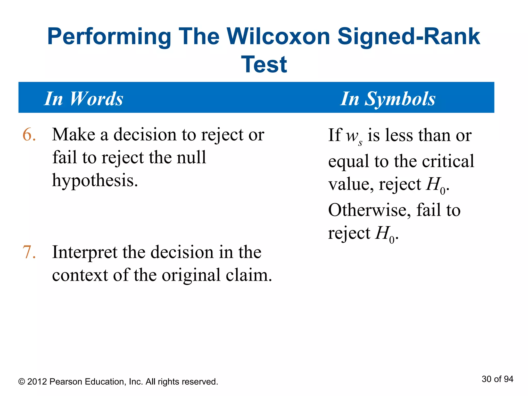
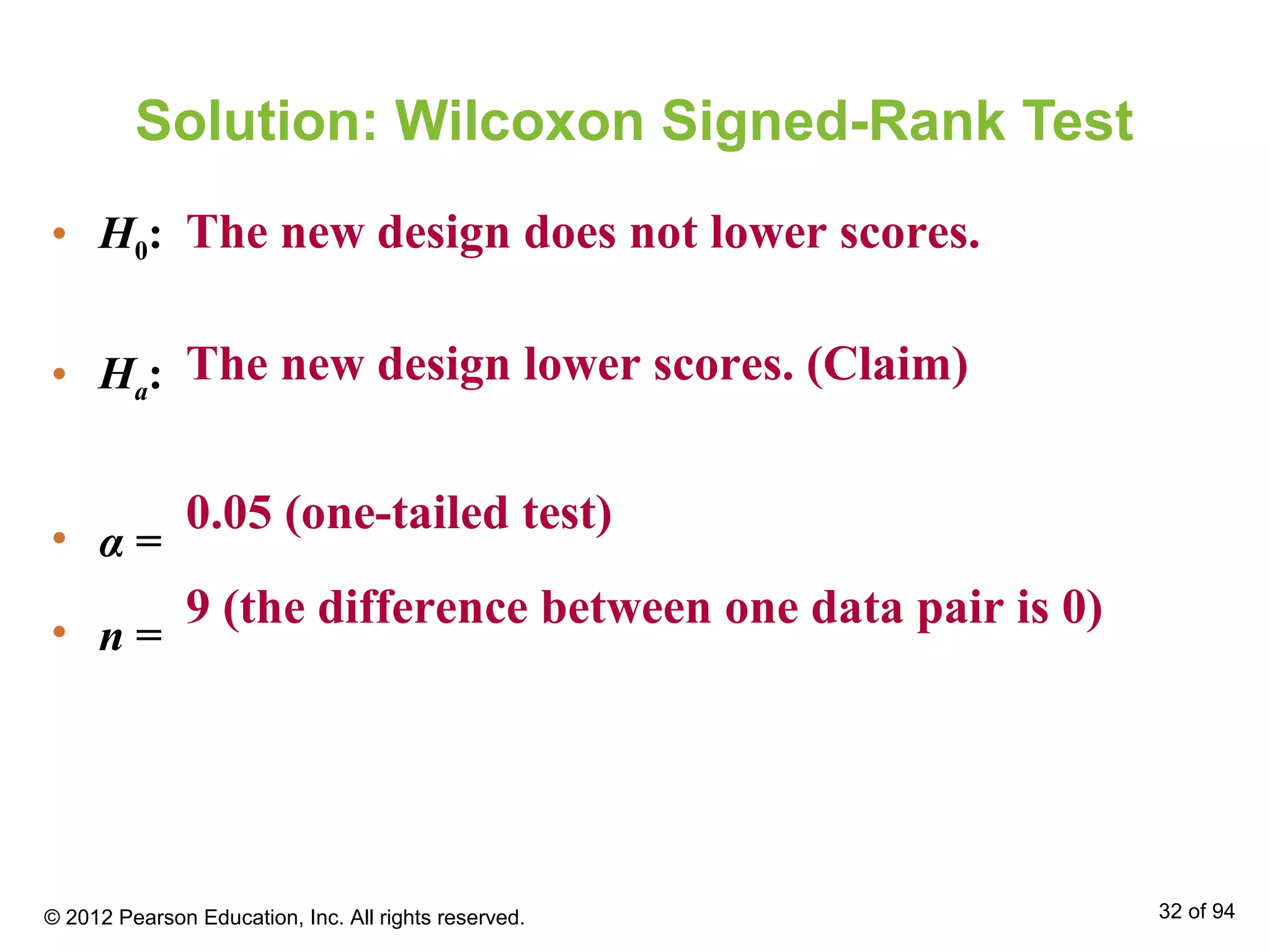
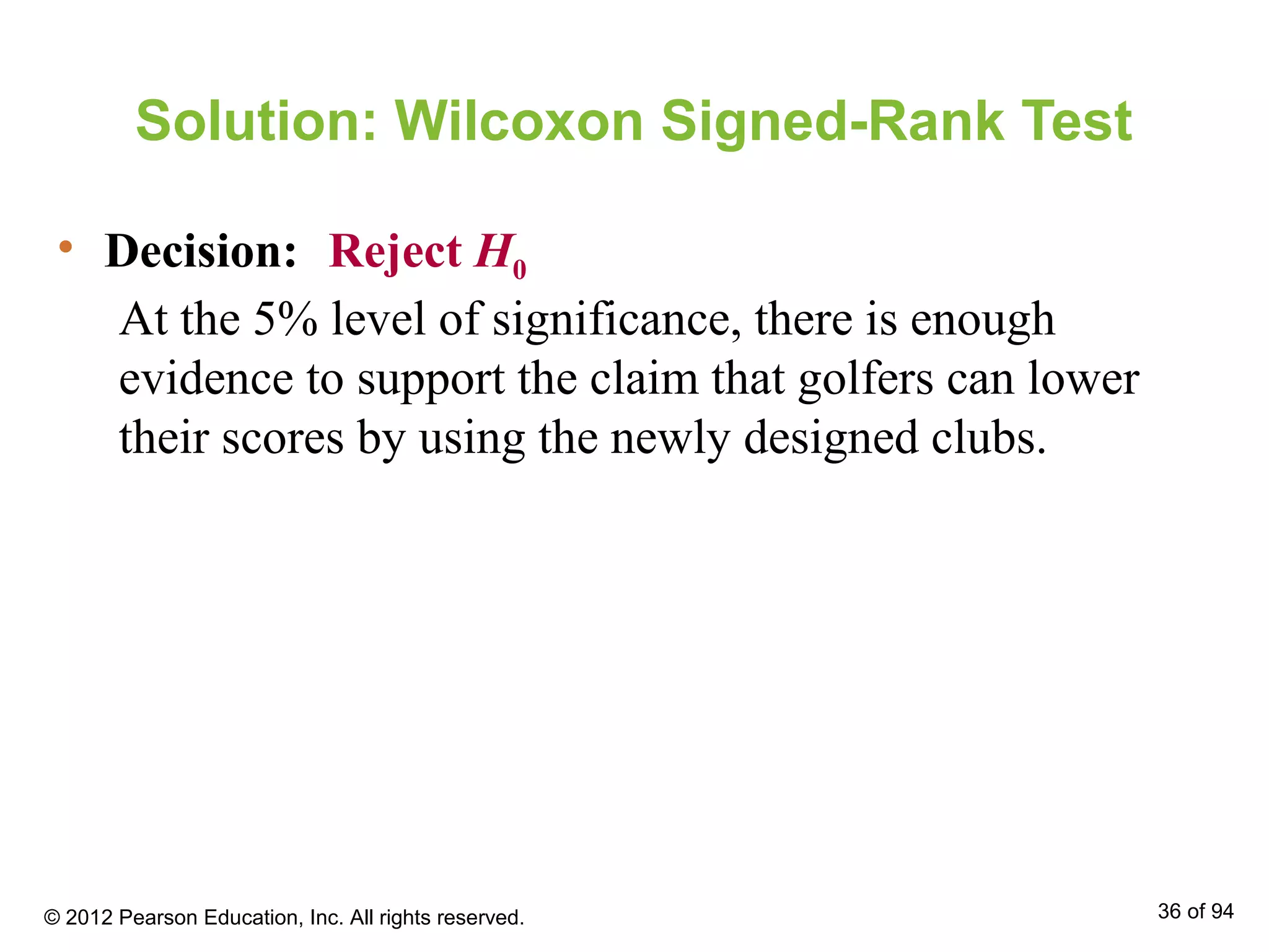
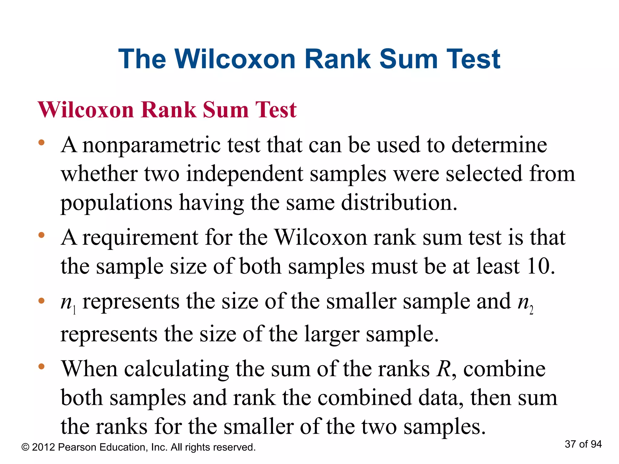
Chapter
Nonparametric Tests
1 of 94
11
© 2012 Pearson Education, Inc.
All rights reserved.

Chapter Outline
• 11.1 The Sign Test
• 11.2 The Wilcoxon Tests
• 11.3 The Kruskal-Wallis Test
• 11.4 Rank Correlation
• 11.5 The Runs Test
© 2012 Pearson Education, Inc. All rights reserved. 2 of 94

Section 11.1
The Sign Test

Section 11.1 Objectives
• Use the sign test to test a population median
• Use the paired-sample sign test to test the difference
between two population medians (dependent
samples)

Nonparametric Test
Nonparametric test
• A hypothesis test that does not require any specific
conditions concerning the shape of the population or
the value of any population parameters.
• Generally easier to perform than parametric tests.
• Usually less efficient than parametric tests (stronger
evidence is required to reject the null hypothesis).

Sign Test for a Population
Median
Sign Test
• A nonparametric test that can be used to test a
population median against a hypothesized value k.
• Left-tailed test:
H0: median ≥ k and Ha: median < k
• Right-tailed test:
H0: median ≤ k and Ha: median > k
• Two-tailed test:
H0: median = k and Ha: median ≠ k

Median
• To use the sign test, each entry is compared with the
hypothesized median k.
 If the entry is below the median, a – sign is
assigned.
 If the entry is above the median, a + sign is
assigned.
 If the entry is equal to the median, 0 is assigned.
• Compare the number of + and – signs.

Median
Test Statistic for the Sign Test
• When n ≤ 25, the test statistic x for the sign test is the
smaller number of + or – signs.
• When n > 25, the test statistic for the sign test is
where x is the smaller number of + or – signs and n is
the sample size (the total number of + or – signs).
( 0.5) 0.5
2
x n
z
n
+ −
=

Performing a Sign Test for a
Population Median
1. Identify the claim. State the
null and alternative hypotheses.
2. Specify the level of
significance.
3. Determine the sample size n by
assigning + signs and – signs to
the sample data.
4. Determine the critical value.
State H0 and Ha.
Identify α.
If n ≤ 25, use Table 8
in Appendix B.
If n > 25, use Table 4
in Appendix B.
n = total number
of + and – signs
In Words In Symbols

Performing a Sign Test for a
Population Median
( 0.5) 0.5
.
2
x n
z
n
+ −
=
If the test statistic is
less than or equal to
the critical value,
reject H0. Otherwise,
fail to reject H0.
5. Calculate the test statistic. If n ≤ 25, use x.
If n > 25, use
In Words In Symbols
6. Make a decision to reject or
fail to reject the null
hypothesis.
7. Interpret the decision in the
context of the original claim.

Example: Using the Sign Test
A website administrator for a company claims that the
median number of visitors per day to the company’s
website is no more than 1500. An employee doubts the
accuracy of this claim. The number of visitors per day
for 20 randomly selected days are listed below. At α =
0.05, can the employee reject the administrator’s claim?
1469 1462 1634 1602 1500
1463 1476 1570 1544 1452
1487 1523 1525 1548 1511
1579 1620 1568 1492 1649

Solution: Using the Sign Test
• H0:
• Ha:
1469 1462 1634 1602 1500
1463 1476 1570 1544 1452
1487 1523 1525 1548 1511
1579 1620 1568 1492 1649
median ≤ 1500 (Claim)
median > 1500
• Compare each data entry with the hypothesized median 1500
– – + + 0
– – + + –
– + + + +
+ + + – +
• There are 7 – signs and 12 + signs
n = 12 + 7 = 19

• α =
• Critical Value: Use Table 8 (n ≤ 25)
0.05
Critical value is 5

• Decision: Fail to reject H0
At the 5% level of significance, there is not enough
evidence for the employee to reject the website
administrator’s claim that the median number of
visitors per day to company’s website is no more
than 1500.
• Test Statistic:
x = 7 (n ≤ 25; use smaller number of + or – signs)

Example: Using the Sign Test
An organization claims that the median annual
attendance for museums in U.S. is at least 39,000. A
random sample of 125 museums reveals that the annual
attendances for 79 museums were less than 39,000, the
annual attendances for 42 museums were more than
39,000, and and the annual attendances for 4 museums
were 39,000. At α = 0.01, is there enough evidence to
reject the organization’s claim? (Adapted from American
Association of Museums)

• H0:
• Ha:
• α =
• Critical value:
median ≥ 39,000 (Claim)
median < 39,000
0.01
n > 25
• Test Statistic:
• Decision:
There are 79 – signs
and 42 + signs.
n = 79 + 42 = 121
x = 42
z =
(42 + 0.5) − 0.5(121)
121
2
=
−18
5.5
≈ −3.27
At the 1% level of significance there is enough
evidence to reject the claim that the median annual
attendance for museums in the U.S. is at least 39,000.
Reject H0

The Paired-Sample Sign Test
Paired-sample sign test
• Used to test the difference between two population
medians when the populations are not normally
distributed.
• For the paired-sample sign test to be used, the
following must be true.
1. A sample must be randomly selected from each
population.
2. The samples must be dependent (paired).
• The difference between corresponding data entries is
found and the sign of the difference is recorded.

Performing The Paired-Sample Sign Test
1. Identify the claim. State the null
and alternative hypotheses.
2. Specify the level of significance.
3. Determine the sample size n by
finding the difference for each
data pair. Assign a + sign for a
positive difference, a – sign for a
negative difference, and a 0 for
no difference.
State H0 and Ha.
Identify α.
n = total number
of + and – signs
In Words In Symbols

Performing The Paired-Sample Sign Test
If the test statistic is
less than or equal to
the critical value,
reject H0.
Otherwise, fail to
reject H0.
5. Find the test statistic. x = smaller number
of + and – signs
Use Table 8 in
Appendix B.
In Words In Symbols
hypothesis.

Example: Paired-Sample Sign Test
A psychologist claims that the number of repeat
offenders will decrease if first-time offenders complete
a particular rehabilitation course. You randomly select
10 prisons and record the number of repeat offenders
during a two-year period. Then, after first-time
offenders complete the course, you record the number
of repeat offenders at each prison for another two-year
period. The results are shown on the next slide. At
α = 0.025, can you support the psychologist’s claim?

Example: Paired-Sample Sign Test
Prison 1 2 3 4 5 6 7 8 9 10
Before 21 34 9 45 30 54 37 36 33 40
After 19 22 16 31 21 30 22 18 17 21
Solution:
• H0:
• Ha:
The number of repeat offenders will not
decrease.
The number of repeat offenders will decrease.
(Claim)
Sign + + – + + + + + + +
• Determine the sign of the difference between the
“before” and “after” data.

Solution: Paired-Sample Sign Test
• α =
• n =
• Critical value:
Sign + + – + + + + + + +
1 + 9 = 10
0.025 (one-tailed)
Critical value is 1

Solution: Paired-Sample Sign Test
• Test Statistic:
• Decision:
Sign + + – + + + + + + +
x = 1 (the smaller number of + or – signs)
Reject H0
At the 2.5% level of significance, there is enough
evidence to support the psychologist’s claim that
the number of repeat offenders will decrease.

Section 11.1 Summary
• Used the sign test to test a population median
• Used the paired-sample sign test to test the difference
between two population medians (dependent
samples)

Section 11.2
The Wilcoxon Tests

• Use the Wilcoxon signed-rank test to determine if two
dependent samples are selected from populations
having the same distribution
• Use the Wilcoxon rank sum test to determine if two
independent samples are selected from populations

The Wilcoxon Signed-Rank Test
Wilcoxon Signed-Rank Test
• A nonparametric test that can be used to determine
whether two dependent samples were selected from
populations having the same distribution.
• Unlike the sign test, it considers the magnitude, or
size, of the data entries.

Performing The Wilcoxon Signed-Rank
Test
3. Determine the sample size n,
which is the number of pairs of
data for which the difference is
not 0.
State H0 and Ha.
Identify α.
In Words In Symbols
Use Table 9 in
Appendix B.

Test
5. Calculate the test statistic ws.
a. Complete a table using the
headers listed at the right.
b. Find the sum of the positive
ranks and the sum of the
negative ranks.
c. Select the smaller of absolute
values of the sums.
Headers: Sample 1,
Sample 2,
Difference,
Absolute value,
Rank, and Signed
rank. Signed rank
takes on the same
sign as its
corresponding
difference.
In Words In Symbols

Test
hypothesis.
If ws is less than or
equal to the critical
value, reject H0.
Otherwise, fail to
reject H0.
In Words In Symbols

Example: Wilcoxon Signed-Rank Test
A golf club manufacturer believes that golfers can lower
their score by using the manufacturer’s newly designed
golf clubs. The scores of 10 golfers while using the old
design and while using the new design are shown in the
table below. At α = 0.05, can you support the
manufacturer’s claim?
Golfer 1 2 3 4 5 6 7 8 9 10
Score (old
design)
89 84 96 74 91 85 95 82 92 81
Score (new
design)
83 83 92 76 91 80 87 85 90 77

Solution: Wilcoxon Signed-Rank Test
• H0:
• Ha:
• α =
• n =
The new design does not lower scores.
The new design lower scores. (Claim)
0.05 (one-tailed test)
9 (the difference between one data pair is 0)

• Critical Value
Table 9
Critical value is 8

Score
(old
design)
Score
(new
design)
Difference
Absolute
value
Rank
Signed
rank
89 83 6 6 8 8
84 83 1 1 1 1
96 92 4 4 5.5 5.5
74 76 –2 2 2.5 –2.5
91 91 0 0 _ _
85 80 5 5 7 7
95 87 8 8 9 9
82 85 –3 3 4 –4
92 90 2 2 2.5 2.5
81 77 4 4 5.5 5.5
• Test Statistic:

• Test Statistic:
The sum of the negative ranks is:
–2.5 + (–4) = –6.5
The sum of the positive ranks is:
8 + 1 + 5.5 + 7 + 9 + 2.5 + 5.5 = 38.5
ws = 6.5 (the smaller of the absolute value of these
two sums: |–6.5| < |38.5|)

• Decision: Reject H0
At the 5% level of significance, there is enough
evidence to support the claim that golfers can lower
their scores by using the newly designed clubs.

The Wilcoxon Rank Sum Test
Wilcoxon Rank Sum Test
whether two independent samples were selected from
populations having the same distribution.
• A requirement for the Wilcoxon rank sum test is that
the sample size of both samples must be at least 10.
• n1 represents the size of the smaller sample and n2
represents the size of the larger sample.
• When calculating the sum of the ranks R, combine
both samples and rank the combined data, then sum
the ranks for the smaller of the two samples.

Test Statistic for The Wilcoxon Rank Sum
Test
• Given two independent samples, the test statistic z
for the Wilcoxon rank sum test is
R
R
R
z
µ
σ
−
=
( )1 1 2 1
2R
n n n
µ
+ +
= ( )1 2 1 2 1
12R
n n n n
σ
+ +
=
where
R = sum of the ranks for the smaller sample,
and

Performing The Wilcoxon Rank Sum Test
3. Determine the critical value(s)
and the rejection region(s).
4. Determine the sample sizes.
State H0 and Ha.
Identify α.
In Words In Symbols
Use Table 4 in
Appendix B.
n1 ≤ n2

5. Find the sum of the ranks for the
smaller sample.
a. List the combined data in
ascending order.
b. Rank the combined data.
c. Add the sum of the ranks for
the smaller sample.
R
In Words In Symbols

6. Calculate the test statistic
and sketch the sampling
distribution.
hypothesis.
In Words In Symbols
If z is in the rejection
region, reject H0.
Otherwise, fail to
reject H0.
R
R
R
z
µ
σ
−
=

Example: Wilcoxon Rank Sum Test
The table shows the earnings (in thousands of dollars)
of a random sample of 10 male and 12 female
pharmaceutical sales representatives. At α = 0.10, can
you conclude that there is a difference between the
males’ and females’ earnings?
Male
earnings
78 93 114 101 98 94 86 95 117 99
Female
earnings
86 77 101 93 85 98 91 87 84 97 100 90

Solution: Wilcoxon Rank Sum Test
• H0:
• Ha:
There is no difference between the males’ and
the females’ earnings.
There is a difference between the males’ and
the females’ earnings. (Claim)
0.10 (two-tailed test)• α =
• Rejection Region:
z
0–1. 645
0.05
1.645
0.05

To find the values of R, μR, and σR, construct a table that
shows the combined data in ascending order and the
corresponding ranks.
Ordered
data
Sample Rank
77 F 1
78 M 2
84 F 3
85 F 4
86 M 5.5
86 F 5.5
87 F 7
90 F 8
91 F 9
93 M 10.5
93 F 10.5
Ordered
data
Sample Rank
94 M 12
95 M 13
97 F 14
98 M 15.5
98 F 15.5
99 M 17
100 F 18
101 M 19.5
101 F 19.5
114 M 21
117 M 22

• Because the smaller sample is the sample of males, R
is the sum of the male rankings.
R = 2 + 5.5 + 10.5 + 12 + 13 + 15.5 + 17 + 19.5 +21 + 22
= 138
• Using n1 = 10 and n2 = 12, we can find μR and σR.
( ) ( )1 1 2 1 10 10 12 1
115
2 2R
n n n
µ
+ + + +
= = =
σR
=
n1
n2
n1
+ n2
+1( )
12
=
(10)(12) 10 +12 +1( )
12
≈15.17

• α =
• H0:
• Ha:
no difference in
earnings.
difference in
earnings.
0.10
z
0–1.645
0.05
1.645
0.05
138 115
15.17
1.52
R
R
R
z
µ
σ
− −
= ≈
≈
• Decision:
At the 10% level of
significance, there is not
enough evidence to conclude
that there is a difference
between the males’ and
females’ earnings.
• Test Statistic
Fail to reject H0
1.52

• Used the Wilcoxon signed-rank test to determine if
two dependent samples are selected from populations
• Used the Wilcoxon rank sum test to determine if two
independent samples are selected from populations

Section 11.3
The Kruskal-Wallis Test

• Use the Kruskal-Wallis test to determine whether
three or more samples were selected from populations

Kruskal-Wallis test
whether three or more independent samples were
selected from populations having the same
distribution.
• The null and alternative hypotheses for the Kruskal-
Wallis test are as follows.
H0: There is no difference in the distribution of the
populations.
Ha: There is a difference in the distribution of the
populations.

• Two conditions for using the Kruskal-Wallis test are
• Each sample must be randomly selected
• The size of each sample must be at least 5.
• If these conditions are met, the test is approximated
by a chi-square distribution with k – 1 degrees of
freedom where k is the number of samples.

Test Statistic for the Kruskal-Wallis Test
• Given three or more independent samples, the test
statistic H for the Kruskal-Wallis test is
22 2
1 2
1 2
12
... 3( 1)
( 1)
k
k
RR R
H N
N N n n n
 
= + + + − + ÷+  
where
k represents the number of samples,
ni is the size of the ith
sample,
N is the sum of the sample sizes,
Ri is the sum of the ranks of the ith
sample.

Performing a Kruskal-Wallis Test
1. Identify the claim. State the
null and alternative
hypotheses.
significance.
3. Identify the degrees of
freedom
4. Determine the critical value
and the rejection region.
State H0 and Ha.
Identify α.
In Words In Symbols
Use Table 6 in
Appendix B.
d.f. = k – 1

5. Find the sum of the ranks
for each sample.
a. List the combined data
in ascending order.
b. Rank the combined data.
5. Calculate the test statistic.
In Words In Symbols
H =
12
N(N +1)
⋅
R1
2
n1
+
R2
2
n2
+ ...+
Rk
2
nk





 − 3(N +1)

7. Make a decision to reject
or fail to reject the null
hypothesis.
8. Interpret the decision in
the context of the original
claim.
In Words In Symbols
If H is in the
rejection region,
reject H0.
Otherwise, fail to
reject H0.

Example: Kruskal-Wallis Test
You want to compare the number of crimes reported in
three police precincts in a city. To do so, you randomly
select 10 weeks for each precinct and record the number
of crimes reported. The results are shown in the table in
next slide. At α = 0.01, can you conclude that the
distributions of crimes reported in the three police
precincts are different?

Example: Kruskal-Wallis Test
Number of Crimes Reported for the week
101st
Precinct
(Sample 1)
106th
Precinct
(Sample 2)
113th
Precinct
(Sample 3)
60 65 69
52 55 51
49 64 70
52 66 61
50 53 67
48 58 65
57 50 62
45 54 59
44 70 60
56 62 63

• α =
• d.f. =
Solution: Kruskal-Wallis Test
• H0:
• Ha:
There is no difference in the number of crimes
reported in the three precincts.
There is a difference in the number of crimes
reported in the three precincts. (Claim)
0.01
k – 1 = 3 – 1 = 2

Ordered
Data Sample Rank
44 101st
1
45 101st
2
48 101st
3
49 101st
4
50 101st
5.5
50 106th
5.5
51 113th
7
52 101st
8.5
52 101st
8.5
53 106th
10
Ordered
Data Sample Rank
54 106th
11
55 106th
12
56 101st
13
57 101st
14
58 106st 15
59 113th
16
60 101st
17.5
60 113th
17.5
61 113th
19
62 106th
20.5
Ordered
Data Sample Rank
62 113th
20.5
63 113th
22
64 106th
23
65 106th
24.5
65 113th
24.5
66 106th
26
67 113th
27
69 113th
28
70 106th
29.5
70 113th
29.5
The table shows the combined data listed in ascending
order and the corresponding ranks.

The sum of the ranks for each sample is as follows.
R1 = 1 + 2 + 3 + 4 + 5.5 + 8.5 + 8.5 + 13 + 14 + 17.5
= 77
R2 = 5.5 + 10 + 11 + 12 + 15 + 20.5 + 23 + 24.5 + 26 + 29.5
= 177
R3 = 7 + 16 + 17.5 + 19 + 20.5 + 22 + 24.5 + 27 + 28 + 29.5
= 211
2 2 2
22 2
1 2
1 2
12 77 177 211
3(30 1) 12.521
3
12
..
0(30 1) 10 10 10
. 3( 1)
( 1)
k
k
RR R
H N
N N n n n
 
= + + − + ≈ ÷+  
 
= + + + − + ÷+  

• H0:
• Ha:
no difference in
number of crimes
difference in
number of crimes
0.01• α =
• d.f. =
3 – 1 = 2
• Decision:
At the 1% level of
significance, there is enough
evidence to support the claim
that there is a difference in
the number of crimes
reported in the three police
precincts.
• Test Statistic
Reject H0
H ≈ 12.521

• Used the Kruskal-Wallis test to determine whether
three or more samples were selected from populations

Section 11.4
Rank Correlation

• Use the Spearman rank correlation coefficient to
determine whether the correlation between two
variables is significant

The Spearman Rank Correlation
Coefficient
Spearman Rank Correlation Coefficient
• A measure of the strength of the relationship between
two variables.
• Nonparametric equivalent to the Pearson correlation
coefficient.
• Calculated using the ranks of paired sample data
entries.
• Denoted rs

Coefficient
Spearman rank correlation coefficient rs
• The formula for the Spearman rank correlation
coefficient is
where n is the number of paired data entries
d is the difference between the ranks of a
paired data entry.
2
2
6
1
( 1)s
d
r
n n
∑
= −
−

Coefficient
• The values of rs range from –1 to 1, inclusive.
 If the ranks of corresponding data pairs are
identical, rs is equal to +1.
 If the ranks are in “reverse” order, rs is equal to –1.
 If there is no relationship, rs is equal to 0.
• To determine whether the correlation between
variables is significant, you can perform a hypothesis
test for the population correlation coefficient ρs.

Coefficient
• The null and alternative hypotheses for this test are as
follows.
H0: ρs = 0 (There is no correlation between the
variables.)
Ha: ρs ≠ 0 (There is a significant correlation between
the variables.)

Testing the Significance of the Spearman
Rank Correlation Coefficient
1. State the null and alternative
hypotheses.
significance.
4. Find the test statistic.
State H0 and Ha.
Identify α.
In Words In Symbols
Use Table 10 in
Appendix B.
2
2
6
1
( 1)s
d
r
n n
∑
= −
−

Testing the Significance of the Spearman
Rank Correlation Coefficient
hypothesis.
context of the original
claim.
In Words In Symbols
If |rs| is greater
than the critical
value, reject H0.
Otherwise, fail to
reject H0.

Example: The Spearman Rank
Correlation Coefficient
The table shows the school
enrollments (in millions) at all
levels of education for males and
females from 2000 to 2007. At α =
0.05, can you conclude that there is
a correlation between the number
of males and females enrolled in
school? (Source: U.S. Census Bureau)
Year Male Female
2000 35.8 36.4
2001 36.3 36.9
2002 36.8 37.3
2003 37.3 37.6
2004 37.4 38.0
2005 37.4 38.4
2006 37.2 38.0
2007 37.6 38.4

• α =
• n =
• Critical value:
Solution: The Spearman Rank
• H0:
• Ha:
ρs = 0 (no correlation between the number of males
and females enrolled in school)
ρs ≠ 0 (correlation between the number of males and
females enrolled in school) (Claim)
0.05
Table 10
8
The critical value
is 0.738

Male Rank Female Rank d d2
35.8 1 36.4 1 0 0
36.3 2 36.9 2 0 0
36.8 3 37.3 3 0 0
37.3 5 37.6 4 1 1
37.4 6.5 38.0 5.5 1 1
37.4 6.5 38.4 7.5 –1 1
37.2 4 38.0 5.5 –1.5 2.25
37.6 8 38.4 7.5 0.5 0.25
Σd2
= 5.5

• α =
• n =
• Critical value:
• H0:
• Ha:
ρs = 0
ρs ≠ 0
0.05
8
The critical value
is 0.738
• Decision:
At the 5% level of significance,
there is enough evidence to
conclude that there is a
correlation between the number
of males and females enrolled in
school.
• Test Statistic
Reject H0
2
2
2
6
1
( 1)
6(5.5)
1 0.935
8(8 1)
s
d
r
n n
∑
= −
−
= − ≈
−

• Used the Spearman rank correlation coefficient to
determine whether the correlation between two
variables is significant

Section 11.5
The Runs Test

• Use the runs test to determine whether a data set is
random

The Runs Test for Randomness
• A run is a sequence of data having the same
characteristic.
• Each run is preceded by and followed by data with a
different characteristic or by no data at all.
• The number of data in a run is called the length of the
run.

Example: Finding the Number of Runs
A liquid-dispensing machine has been designed to fill
one-liter bottles. A quality control inspector decides
whether each bottle is filled to an acceptable level and
passes inspection (P) or fails inspection (F). Determine
the number of runs for the sequence and find the length
of each run.
P P F F F F P F F F P P P P P P
P P F F F F P F F F P P P P P PLength
of run:
There are 5 runs.
2 4 1 3 6
Solution:

Runs Test for Randomness
Runs Test for Randomness
whether a sequence of sample data is random.
• The null and alternative hypotheses for this test are as
follows.
H0: The sequence of data is random.
Ha: The sequence of data is not random.

Test Statistic for the Runs Test
• When n1 ≤ 20 and n2 ≤ 20, the test statistic for the runs
test is G, the number of runs.
G
G
G
z
µ
σ
−
=
1 2 1 2 1 2 1 2
2
1 2 1 2 1 2
2 2 (2 )
1 and
( ) ( 1)G G
n n n n n n n n
n n n n n n
µ σ
− −
= + =
+ + + −
• When n1 > 20 or n2 > 20, the test statistic for the
runs test is
where

Performing a Runs Test for Randomness
Determine n1, n2, and
G.
significance. (Use α = 0.05 for
the runs test.)
3. Determine the number of data
that have each characteristic
and the number of runs.
State H0 and Ha.
Identify α.
In Words In Symbols

4. Determine the critical
values.
5. Calculate the test statistic.
.G
G
G
z
µ
σ
−
=
If n1 ≤ 20 and n2 ≤ 20, use
G.
If n1 > 20 or n2 > 20, use
In Words In Symbols
If n1 ≤ 20 and n2 ≤ 20, use
Table 12 in Appendix B.
If n1 > 20 or n2 > 20, use
Table 4 in Appendix B.

hypothesis.
context of the original
claim.
If G ≤ the lower
critical value, or if
G ≥ the upper critical
value, reject H0.
Otherwise, fail to
reject H0.
In Words In Symbols

Example: Using the Runs Test
As people enter a concert, an usher records where they
are sitting. The results for 13 people are shown, where L
represents a lawn seat and P represents a pavilion seat.
At α = 0.05, can you conclude that the sequence of seat
locations is not random?
L L L P P L P P P L L P L

Solution: Using the Runs Test
L L L P P L P P P L L P L
• H0:
• Ha:
The sequence of seat locations is random.
The sequences of seat locations is not random. (Claim)
• n1 = number of L’s =
• n2 = number of P’s =
• G = number of runs =
• α =
• Critical value:
7
7
6
0.05
Because n1 ≤ 20, n2 ≤ 20, use Table 12

• Critical value:
• n1 = 7 n2 = 6 G = 7
The lower
critical value is
3 and the upper
critical value is
12.

• H0:
• Ha:
random
not random
• n1 = n2 =
• G =
• α =
• Critical value:
7
7
6
0.05
lower critical value = 3
upper critical value =12
• Decision:
At the 5% level of
significance, there is not
enough evidence to support
the claim that the sequence of
seat locations is not random.
So, it appears that the
sequence of seat locations is
random.
• Test Statistic:
Fail to Reject H0
G = 7

Example: Using the Runs Test
You want to determine whether the selection of recently
hired employees in a large company is random with
respect to gender. The genders of 36 recently hired
employees are shown below. At α = 0.05, can you
conclude that the selection is not random?
M M F F F F M M M M M M
F F F F F M M M M M M M
F F F M M M M F M M F M

M M F F F F M M M M M M
F F F F F M M M M M M M
F F F M M M M F M M F M
• H0:
• Ha:
The selection of employees is random.
The selection of employees is not random.
• n1 = number of F’s =
• n2 = number of M’s =
• G = number of runs =
14
11
22

• H0:
• Ha:
random
not random
• n1 = n2 =
• G =
• α =
• Critical value:
14
11
22
0.05 • Decision:
• Test Statistic:
n2 > 20, use Table 4
z
0–1.96
0.025
1.96
0.025

G
G
G
z
µ
σ
−
= ≈
1 2
1 2
2
1 =G
n n
n n
µ = +
+
1 2 1 2 1 2
2
1 2 1 2
2 (2 )
( ) ( 1)G
n n n n n n
n n n n
σ
− −
=
+ + −
2(14)(22)
1 18.11
14 22
+ ≈
+
2
2(14)(22)[2(14)(22) 14 22)
2.81
(14 22) (14 22 1)
− −
= ≈
+ + −
11 18.11
2.53
2.81
−
≈ −

• H0:
• Ha:
random
not random
• n1 = n2 =
• G =
• α =
• Critical value:
14
11
22
0.05
• Decision:
• Test Statistic:
z
0–1.96
0.025
1.96
0.025
–2.53
You have enough evidence at
the 5% level of significance
to support the claim that the
selection of employees with
respect to gender is not
random.
Reject H0
z ≈ –2.53

• Used the runs test to determine whether a data set is
random

Les5e ppt 11

More Related Content

What's hot

Viewers also liked

Similar to Les5e ppt 11

More from Subas Nandy

Recently uploaded

Les5e ppt 11