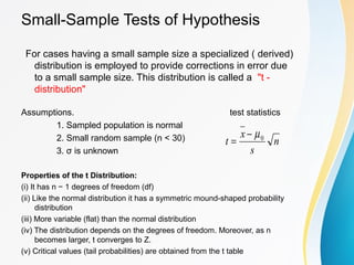
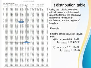
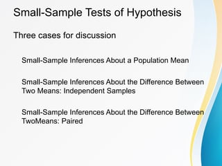
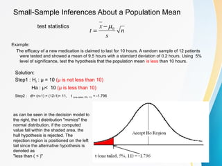
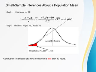
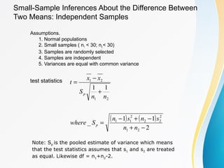
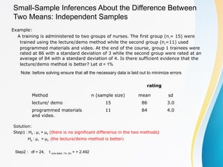
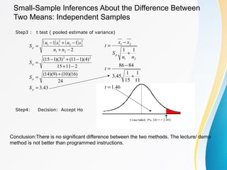
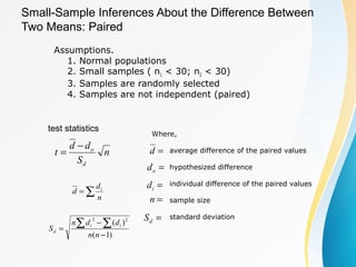
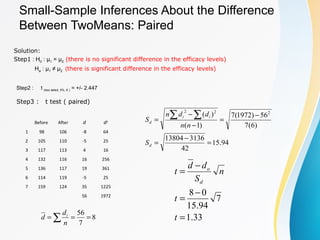
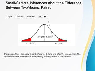
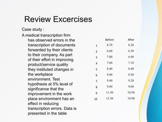
The document discusses small sample tests of hypotheses. It explains that for small sample sizes (n<30), a t-distribution is used instead of the normal distribution to account for the small sample size. There are three cases discussed for small sample tests: testing a population mean, comparing the means of two independent samples, and comparing the means of two paired samples. For each case, the assumptions, test statistic (involving a t-distribution), and an example are provided.

1. Statistical Test of
Hypothesis ( Part 2)

2. Small-Sample Tests of Hypothesis
For cases having a small sample size a specialized ( derived)
distribution is employed to provide corrections in error due
to a small sample size. This distribution is called a "t -
distribution"
Assumptions. test statistics
1. Sampled population is normal
2. Small random sample (n < 30)
3. σ is unknown
Properties of the t Distribution:
(i) It has n − 1 degrees of freedom (df)
(ii) Like the normal distribution it has a symmetric mound-shaped probability
distribution
(iii) More variable (flat) than the normal distribution
(iv) The distribution depends on the degrees of freedom. Moreover, as n
becomes larger, t converges to Z.
(v) Critical values (tail probabilities) are obtained from the t table
n
s
x
t 0µ−
=

3. t distribution table
Using the t distribution table,
critical values are determined
given the form of the alternative
hypothesis the level of
confidence, and the degree of
freedom
Example:
Find the critical values of t given
that:
a) Ha: ≠ , α = 0.05 df =12
t(two tailed,α,df,) = +/- 2.179
b) Ha: > , α = 0.01 df =29
t(one tailed,α,df,) = + 2.462

4. Small-Sample Tests of Hypothesis
Three cases for discussion
Small-Sample Inferences About a Population Mean
Small-Sample Inferences About the Difference Between
Two Means: Independent Samples
Small-Sample Inferences About the Difference Between
TwoMeans: Paired

5. Small-Sample Inferences
About a Population Mean

6. Small-Sample Inferences About a Population Mean
Example:
The efficacy of a new medication is claimed to last for 10 hours. A random sample of 12 patients
were tested and showed a mean of 9.5 hours with a standard deviation of 0.2 hours. Using 5%
level of significance, test the hypothesis that the population mean is less than 10 hours.
n
s
x
t 0µ−
=
test statistics
Solution:
Step1 : H0 : μ = 10 (μ is not less than 10)
Ha : μ< 10 (μ is less than 10)
Step2 : df= (n-1) = (12-1)= 11, t (one tailed, 5%, 11) = -1.796
as can be seen in the decision model to
the right, the t distribution "mimics" the
normal distribution, if the computed
value fall within the shaded area, the
hull hypothesis is rejected. The
rejection region is positioned on the left
tail since the alternative hypothesis is
denoted as
"less than ( < )"

7. Small-Sample Inferences About a Population Mean
Step3 : t test since n ≤ 30
Step4: Decision: Reject Ho, Accept Ha
Conclusion: Th efficacy of a new medication is less than 10 hours.
-8.66012
2.0
10)5.9(0
=
−
=
−
= n
s
x
t
µ

8. Review Excercises
Case Study:
A panel survey was conducted to by the National
Population Commission to study the general effects
of aging on the sociological and physiological well
being of senior citizens living in selected urban
areas in Metro Manila. 24 senior citizens in
Barangay Nagkaisa participated in the study. The
life expectancy of the participants were measured at
78.23 years with sd of 7.2 years.
If the national life expectancy is 72 years is there
sufficient evidence that the respondents lived
longer? Level of significance is at 5%.

9. Small-Sample Inferences
About the Difference
Between Two Means:
Independent Samples

10. Small-Sample Inferences About the Difference Between
Two Means: Independent Samples
Assumptions.
1. Normal populations
2. Small samples ( n1 < 30; n2 < 30)
3. Samples are randomly selected
4. Samples are independent
5. Variances are equal with common variance
( ) ( )
2
11
_
11
21
2
22
2
11
21
21
−+
−+−
=
+
−
=
nn
snsn
Swhere
nn
S
xx
t
p
p
test statistics
Note: Sp is the pooled estimate of variance which means
that the test statistics assumes that s1 and s2 are treated
as equal. Likewise df = n1+n2-2.

11. Small-Sample Inferences About the Difference Between
Two Means: Independent Samples
Example:
A training is administered to two groups of nurses. The first group (n1= 15) were
trained using the lecture/demo method while the second group (n2=11) used
programmed materials and video. At the end of the course, group 1 trainees were
rated at 86 with a standard deviation of 3 while the second group were rated at an
average of 84 with a standard deviation of 4. Is there sufficient evidence that the
lecture/demo method is better? Let α = 1%
Note: before solving ensure that all the necessary data is laid out to minimize errors
rating
Method n (sample size) mean sd
lecture/ demo 15 86 3.0
programmed materials
and video.
11 84 4.0
Solution:
Step1 : H0 : μ1 = μ2 (there is no significant difference in the two methods)
Ha : μ1 > μ2 (the lecture/demo method is better)
Step2 : df = 24, t (one tailed, 1%, 24) = + 2.492

12. Small-Sample Inferences About the Difference Between
Two Means: Independent Samples
( ) ( )
43.3
24
)16)(10()9)(14(
21115
)4)(111()3)(115(
2
11
22
21
2
22
2
11
=
+
=
−+
−+−
=
−+
−+−
=
p
p
p
p
S
S
S
nn
snsn
S
Step3 : t test ( pooled estimate of variance)
46.1
11
1
15
1
45.3
8486
11
21
21
=
+
−
=
+
−
=
t
t
nn
S
xx
t
p
Step4: Decision: Accept Ho
Conclusion:There is no significant difference between the two methods. The lecture/ demo
method is not better than programmed instructions.

13. Review Excercises
Refer to the results in the case study
"magnets and pain relief"
pain before
(Score_1)
pain after
(Score_2)
n (sample
size)
mean sd mean sd
Active
Magnet
29 9.6206 0.7277 4.3793 3.1443
Inactive
Placebo
21 9.5238 0.8728 8.4285 1.8593
Test the hypothesis (alpha= 1%):
a) The two groups has comparable pain levels before the
"magnets" were used.
b) Bioflex magnets were more effective in pain management

14. Small-Sample Inferences
About the Difference
Between Two Means:
Paired

15. Where,
average difference of the paired values
hypothesized difference
individual difference of the paired values
sample size
standard deviation
Small-Sample Inferences About the Difference Between
Two Means: Paired
Assumptions.
1. Normal populations
2. Small samples ( n1 < 30; n2 < 30)
3. Samples are randomly selected
4. Samples are not independent (paired)
n
S
dd
t
d
o−
= =d
test statistics
∑=
n
d
d i
)1(
)( 22
−
−
=
∑ ∑
nn
ddn
S ii
d
=od
=id
=n
=dS

16. Small-Sample Inferences About the Difference
Between TwoMeans: Paired
Example:
An intervention program is administered to seven ( 7 ) patients who experienced myocardial infarction or
cardiac surgery. The program involves coaching to improve self efficacy of the participants to perform
a range of activities frequently encountered in daily living ( bathing, walking, dressing up etc). The
design involves 2 weeks of coaching. Self efficacy ratings were taken before and after the coaching
activities.
The results are illustrated in the table below:
Before After
1 98 106
2 105 110
3 117 113
4 132 116
5 136 117
6 114 119
7 159 124
Test the hypothesis that there is a significant difference in the self efficacy ratings at 5% level of
significance.

17. Small-Sample Inferences About the Difference
Between TwoMeans: Paired
Solution:
Step1 : H0 : μ1 = μ2 (there is no significant difference in the efficacy levels)
Ha : μ1 ≠ μ2 (there is significant difference in the efficacy levels)
Step2 : t (two tailed, 5%, 6 ) = +/- 2.447
Before After d d2
1 98 106 -8 64
2 105 110 -5 25
3 117 113 4 16
4 132 116 16 256
5 136 117 19 361
6 114 119 -5 25
7 159 124 35 1225
56 1972
Step3 : t test ( paired)
8
7
56
=== ∑ n
d
d i
94.15
42
313613804
)6(7
56)1972(7
)1(
)( 222
=
−
=
−
=
−
−
=
∑ ∑
d
ii
d
S
nn
ddn
S
33.1
7
94.15
08
=
−
=
−
=
t
t
n
S
dd
t
d
o

18. Small-Sample Inferences About the Difference
Between TwoMeans: Paired
Step4: Decision: Accept Ho t= 1.33
Conclusion:There is no significant difference before and after the intervention. The
intervention was not effective in improving efficacy levels of the patients

19. Review Excercises
Case study :
A medical transcription firm
has observed errors in the
transcription of documents
forwarded by their clients
to their company. As part
of their effort in improving
product/service quality
they instituted changes in
the workplace
environment. Test
hypothesis at 5% level of
significance that the
improvement in the work
place environment has an
effect in reducing
transcription errors. Data is
presented in the table
Before After
1 8.70 8.20
2 6.60 6.30
3 7.00 6.90
4 7.60 7.10
5 8.40 8.40
6 9.00 8.50
7 9.40 9.20
8 9.60 9.60
9 11.30 10.50
10 12.30 10.90

20. End of
Second Part of
the Discussions