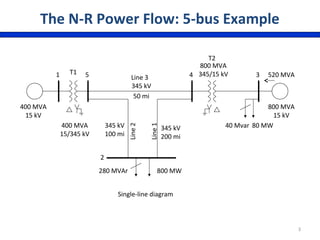
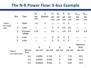
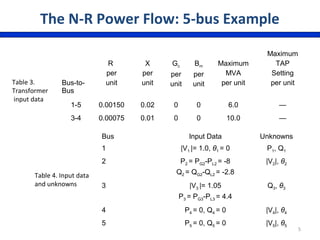
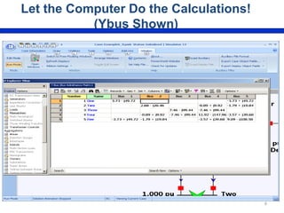
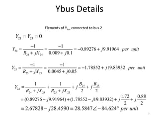
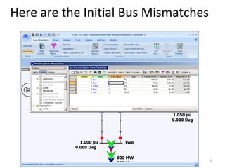
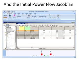
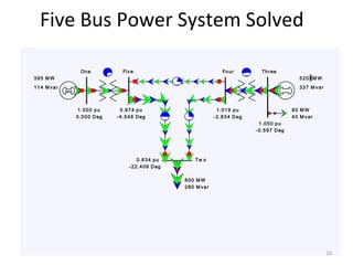
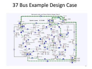
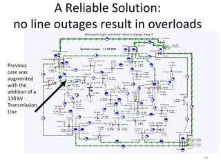
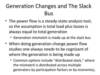
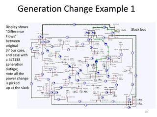
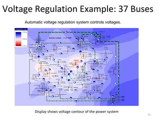
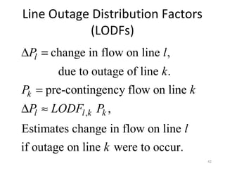
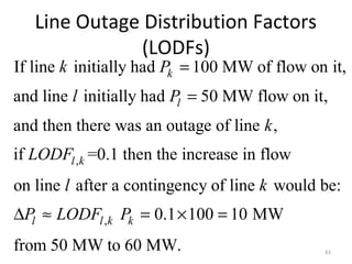
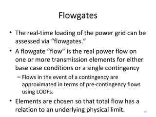
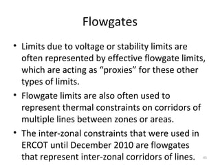
SlideShare a Scribd company logo
EE 369
POWER SYSTEM ANALYSIS
Lecture 14
Power Flow
Tom Overbye and Ross Baldick
1
Announcements
Read Chapter 12, concentrating on sections
12.4 and 12.5.
Homework 12 is 6.43, 6.48, 6.59, 6.61,
12.19, 12.22, 12.20, 12.24, 12.26, 12.28,
12.29; due Tuesday Nov. 25.
2
400 MVA
15 kV
400 MVA
15/345 kV
T1
T2
800 MVA
345/15 kV
800 MVA
15 kV
520 MVA
80 MW40 Mvar
280 MVAr 800 MW
Line 3
345 kV
Line2
Line1
345 kV
100 mi
345 kV
200 mi
50 mi
1 4 3
2
5
Single-line diagram
The N-R Power Flow: 5-bus Example
3
Bus Type
|V|
per
unit
θ
degrees
PG
per
unit
QG
per
unit
PL
per
unit
QL
per
unit
QGmax
per
unit
QGmin
per
unit
1 Slack 1.0 0   0 0  
2 Load   0 0 8.0 2.8  
3 Constant
voltage
1.05  5.2  0.8 0.4 4.0 -2.8
4 Load   0 0 0 0  
5 Load   0 0 0 0  
Table 1.
Bus input
data
Bus-to-
Bus
R
per unit
X
per unit
G
per unit
B
per unit
Maximum
MVA
per unit
2-4 0.0090 0.100 0 1.72 12.0
2-5 0.0045 0.050 0 0.88 12.0
4-5 0.00225 0.025 0 0.44 12.0
Table 2.
Line input data
The N-R Power Flow: 5-bus Example
4
Bus-to-
Bus
R
per
unit
X
per
unit
Gc
per
unit
Bm
per
unit
Maximum
MVA
per unit
Maximum
TAP
Setting
per unit
1-5 0.00150 0.02 0 0 6.0 —
3-4 0.00075 0.01 0 0 10.0 —
Table 3.
Transformer
input data
Bus Input Data Unknowns
1 |V1 |= 1.0, θ1 = 0 P1, Q1
2 P2 = PG2-PL2 = -8
Q2 = QG2-QL2 = -2.8
|V2|, θ2
3 |V3 |= 1.05
P3 = PG3-PL3 = 4.4
Q3, θ3
4 P4 = 0, Q4 = 0 |V4|, θ4
5 P5 = 0, Q5 = 0 |V5|, θ5
Table 4. Input data
and unknowns
The N-R Power Flow: 5-bus Example
5
Let the Computer Do the Calculations!
(Ybus Shown)
6
Ybus Details
02321 == YY
24
24 24
1 1
0.89276 9.91964
0.009 0.1
Y j per unit
R jX j
− −
= = = − +
+ +
25
25 25
1 1
1.78552 19.83932
0.0045 0.05
Y j per unit
R jX j
− −
= = = − +
+ +
24 25
22
24 24 25 25
1 1
2 2
B B
Y j j
R jX R jX
= + + +
+ +
2
88.0
2
72.1
)83932.1978552.1()91964.989276.0( jjjj ++−+−=
unitperj °−∠=−= 624.845847.284590.2867828.2
Elements of Ybus connected to bus 2
7
Here are the Initial Bus Mismatches
8
And the Initial Power Flow Jacobian
9
Five Bus Power System Solved
slack
One
Tw o
ThreeFourFive
A
MVA
A
MVA
A
MVA
A
MVA
A
MVA
1.000 pu 0.974 pu
0.834 pu
1.019 pu
1.050 pu
0.000 Deg - 4.548 Deg
-22.406 Deg
-2.834 Deg
- 0.597 Deg
395 M W
114 M var
520 M W
337 M var
800 M W
280 M var
80 M W
40 M var
10
37 Bus Example Design Case
slack
Metropolis Light and Pow er Electric Design Case 2
SL A C K 3 4 5
SL A C K 1 3 8
R A Y 3 4 5
R A Y 1 3 8
R A Y 6 9
FER N A 6 9
A
MVA
D EM A R 6 9
B L T 6 9
B L T 1 3 8
B O B 1 3 8
B O B 6 9
W O L EN 6 9
SH I M K O 6 9
R O GER 6 9
U I U C 6 9
P ET E6 9
H I SK Y 6 9
T I M 6 9
T I M 1 3 8
T I M 3 4 5
P A I 6 9
GR O SS6 9
H A N N A H 6 9
A M A N D A 6 9
H O M ER 6 9
L A U F6 9
M O R O 1 3 8
L A U F1 3 8
H A L E6 9
P A T T EN 6 9
W EB ER 6 9
B U C K Y 1 3 8
SA V O Y 6 9
SA V O Y 1 3 8
JO 1 3 8 JO 3 4 5
A
MVA
A
MVA
A
MVA
A
MVA
A
MVA
A
MVA
A
MVA
A
MVA
A
MVA
A
MVA
A
MVA
A
MVA
A
MVA
A
MVA
A
MVA
A
MVA
A
MVA
A
MVA
A
MVA
A
MVA
A
MVA
A
MVA
A
MVA
A
MVA
A
MVA
A
MVA
A
MVA
A
MVA
A
MVA
A
MVA
A
MVA
A
MVA
A
MVA
A
MVA
A
MVA
A
MVA
A
MVA
A
MVA
A
MVA
A
MVA
A
MVA
A
MVA
A
MVA
A
MVA
A
MVA
A
MVA
A
MVA
A
MVA
A
MVA
1 .0 3 p u
1 .0 2 p u
1 .0 3 p u
1 .0 3 p u
1 .0 1 p u
1 .0 0 p u
1 .0 1 p u
1 .0 0 p u
1 .0 2 p u
1 .0 1 p u
1 .0 0 p u
1 .0 1 p u
1 .0 1 p u
1 .0 1 p u
1 .0 1 p u
1 .0 2 p u
1 .0 0 p u
1 .0 0 p u
1 .0 2 p u
0 .9 9 p u
0 .9 9 p u
1 .0 0 p u
1 .0 2 p u
1 .0 0 p u
1 .0 1 p u
1 .0 1 p u
1 .0 0 p u 1 .0 0 p u
1 .0 1 p u
1 .0 2 p u
1 .0 2 p u
1 .0 2 p u
1 .0 3 p u
A
MVA
1 .0 2 p u
A
MVA
A
MVA
L Y N N 1 3 8
A
MVA
1 .0 2 p u
A
MVA
1 .0 0 p u
A
MVA
Syst em Losses: 10.70 MW
2 2 0 M W
5 2 M v a r
1 2 M W
3 M v a r
2 0 M W
1 2 M v a r
1 2 4 M W
4 5 M v a r
3 7 M W
1 3 M v a r
1 2 M W
5 M v a r
1 5 0 M W
0 M v a r
5 6 M W
1 3 M v a r
1 5 M W
5 M v a r
1 4 M W
2 M v a r
3 8 M W
3 M v a r
4 5 M W
0 M v a r
2 5 M W
3 6 M v a r
3 6 M W
1 0 M v a r
1 0 M W
5 M v a r
2 2 M W
1 5 M v a r
6 0 M W
1 2 M v a r
2 0 M W
2 8 M v a r
2 3 M W
7 M v a r
3 3 M W
1 3 M v a r
1 5 .9 M v a r 1 8 M W
5 M v a r
5 8 M W
4 0 M v a r
6 0 M W
1 9 M v a r
1 4 .2 M v a r
2 5 M W
1 0 M v a r
2 0 M W
3 M v a r
2 3 M W
6 M v a r 1 4 M W
3 M v a r
4 .9 M v a r
7 .3 M v a r
1 2 .8 M v a r
2 8 .9 M v a r
7 .4 M v a r
0 .0 M v a r
5 5 M W
2 5 M v a r
3 9 M W
1 3 M v a r
1 5 0 M W
0 M v a r
1 7 M W
3 M v a r
1 6 M W
- 1 4 M v a r
1 4 M W
4 M v a r
KYLE6 9
A
MVA
11
Good Power System Operation
• Good power system operation requires that
there be no “reliability” violations (needing to
shed load, have cascading outages, or other
unacceptable conditions) for either the current
condition or in the event of statistically likely
contingencies:
• Reliability requires as a minimum that there be no
transmission line/transformer limit violations and
that bus voltages be within acceptable limits
(perhaps 0.95 to 1.08)
• Example contingencies are the loss of any single
device. This is known as n-1 reliability. 12
Good Power System Operation
• North American Electric Reliability Corporation
now has legal authority to enforce reliability
standards (and there are now lots of them).
• See http://www.nerc.com for details (click on
Standards)
13
Looking at the Impact of Line Outages
slack
Metropolis Light and Pow er Electric Design Case 2
SL A C K 3 4 5
SL A C K 1 3 8
R A Y 3 4 5
R A Y 1 3 8
R A Y 6 9
FER N A 6 9
A
MVA
D EM A R 6 9
B L T 6 9
B L T 1 3 8
B O B 1 3 8
B O B 6 9
W O L EN 6 9
SH I M K O 6 9
RO GER6 9
U I U C 6 9
P ET E6 9
H I SK Y 6 9
T I M 6 9
T I M 1 3 8
T I M 3 4 5
P A I 6 9
GR O SS6 9
H A N N A H 6 9
A M A N DA 6 9
H O M ER 6 9
L A U F6 9
M O R O 1 3 8
L A U F1 3 8
H A L E6 9
P A T T EN 6 9
W EB ER 6 9
B U C K Y 1 3 8
SA V O Y 6 9
SA V O Y 1 3 8
JO 1 3 8 JO 3 4 5
A
MVA
A
MVA
A
MVA
A
MVA
A
MVA
A
MVA
A
MVA
A
MVA
A
MVA
A
MVA
A
MVA
A
MVA
A
MVA
A
MVA
A
MVA
A
MVA
A
MVA
A
MVA
A
MVA
A
MVA
A
MVA
A
MVA
A
MVA
A
MVA
A
MVA
A
MVA
A
MVA
A
MVA
A
MVA
A
MVA
A
MVA
A
MVA
A
MVA
A
MVA
A
MVA
A
MVA
A
MVA
A
MVA
A
MVA
A
MVA
A
MVA
A
MVA
A
MVA
A
MVA
A
MVA
1 .0 3 p u
1 .0 2 p u
1 .0 3 p u
1 .0 3 p u
1 .0 1 p u
1 .0 0 p u
1 .0 1 p u
1 .0 0 p u
1 .0 2 p u
1 .0 1 p u
1 .0 0 p u
1 .0 1 p u
1 .0 1 p u
1 .0 1 p u
1 .0 1 p u
1 .0 2 p u
1 .0 1 p u
1 .0 0 p u
1 .0 2 p u
0 .9 0 p u
0 .9 0 p u
0 .9 4 p u
1 .0 1 p u
0 .9 9 p u
1 .0 0 p u
1 .0 0 p u
1 .0 0 p u 1 .0 0 p u
1 .0 1 p u
1 .0 1 p u
1 .0 2 p u
1 .0 2 p u
1 .0 3 p u
A
MVA
1 .0 2 p u
A
MVA
A
MVA
L Y N N 1 3 8
A
MVA
1 .0 2 p u
A
MVA
1 .0 0 p u
A
MVA
Syst em Losses: 17.61 MW
2 2 7 M W
4 3 M v a r
1 2 M W
3 M v a r
2 0 M W
1 2 M v a r
1 2 4 M W
4 5 M v a r
3 7 M W
1 3 M v a r
1 2 M W
5 M v a r
1 5 0 M W
4 M v a r
5 6 M W
1 3 M v a r
1 5 M W
5 M v a r
1 4 M W
2 M v a r
3 8 M W
9 M v a r
4 5 M W
0 M v a r
2 5 M W
3 6 M v a r
3 6 M W
1 0 M v a r
1 0 M W
5 M v a r
2 2 M W
1 5 M v a r
6 0 M W
1 2 M v a r
2 0 M W
4 0 M v a r
2 3 M W
7 M v a r
3 3 M W
1 3 M v a r
1 6 .0 M v a r 1 8 M W
5 M v a r
5 8 M W
4 0 M v a r
6 0 M W
1 9 M v a r
1 1 .6 M v a r
2 5 M W
1 0 M v a r
2 0 M W
3 M v a r
2 3 M W
6 M v a r 1 4 M W
3 M v a r
4 .9 M v a r
7 .2 M v a r
1 2 .8 M v a r
2 8 .9 M v a r
7 .3 M v a r
0 .0 M v a r
5 5 M W
3 2 M v a r
3 9 M W
1 3 M v a r
1 5 0 M W
4 M v a r
1 7 M W
3 M v a r
1 6 M W
- 1 4 M v a r
1 4 M W
4 M v a r
KYLE6 9
A
MVA
8 0 %
A
MVA
1 3 5 %
A
M VA
1 1 0 %
A
M VA
Opening
one line
(Tim69-
Hannah69)
causes
overloads.
This would
not be
Allowed.
14
Contingency Analysis
Contingency
analysis provides
an automatic
way of looking
at all the
statistically
likely
contingencies. In
this example the
contingency set
is all the single
line/transformer
outages
15
Power Flow And Design
• One common usage of the power flow is to
determine how the system should be modified
to remove contingencies problems or serve new
load
• In an operational context this requires working with
the existing electric grid, typically involving re-
dispatch of generation.
• In a planning context additions to the grid can be
considered as well as re-dispatch.
• In the next example we look at how to remove
the existing contingency violations while serving
new load. 16
An Unreliable Solution:
some line outages result in overloads
slack
Metropolis Light and Pow er Electric Design Case 2
SL A C K 3 4 5
SL A C K 1 3 8
R A Y 3 4 5
R A Y 1 3 8
R A Y 6 9
FER N A 6 9
A
MVA
D EM A R 6 9
B L T 6 9
B L T 1 3 8
B O B 1 3 8
B O B 6 9
W O L EN6 9
SH I M K O 6 9
RO GER 6 9
U I U C 6 9
P ET E6 9
H I SK Y 6 9
T I M 6 9
T I M 1 3 8
T I M 3 4 5
P A I 6 9
GR O SS6 9
H A N NA H 6 9
A M A N DA 6 9
H O M ER 6 9
L A U F6 9
M O R O 1 3 8
L A U F1 3 8
H A L E6 9
P A T T EN 6 9
W EB ER6 9
B U CK Y 1 3 8
SA V O Y 6 9
SA V O Y 1 3 8
JO 1 3 8 JO 3 4 5
A
MVA
A
MVA
A
MVA
A
MVA
A
MVA
A
MVA
A
MVA
A
MVA
A
MVA
A
MVA
A
MVA
A
MVA
A
MVA
A
MVA
A
MVA
A
MVA
A
MVA
A
MVA
A
MVA
A
MVA
A
MVA
A
MVA
A
MVA
A
MVA
A
MVA
A
MVA
A
MVA
A
MVA
A
MVA
A
MVA
A
MVA
A
MVA
A
MVA
A
MVA
A
MVA
A
MVA
A
MVA
A
MVA
A
MVA
A
MVA
A
MVA
A
MVA
A
MVA
A
MVA
A
MVA
A
MVA
A
MVA
A
MVA
1 .0 2 p u
1 .0 1 p u
1 .0 2 p u
1 .0 3 p u
1 .0 1 p u
1 .0 0 p u
1 .0 1 p u
1 .0 0 p u
1 .0 2 p u
1 .0 1 p u
1 .0 0 p u
1 .0 1 p u
1 .0 1 p u
1 .0 1 p u
1 .0 1 p u
1 .0 2 p u
0 .9 9 p u
1 .0 0 p u
1 .0 2 p u
0 .9 7 p u
0 .9 7 p u
0 .9 9 p u
1 .0 2 p u
1 .0 0 p u
1 .0 1 p u
1 .0 1 p u
1 .0 0 p u 1 .0 0 p u
1 .0 1 p u
1 .0 2 p u
1 .0 2 p u
1 .0 2 p u
1 .0 3 p u
A
MVA
1 .0 2 p u
A
MVA
A
MVA
L Y N N1 3 8
A
MVA
1 .0 2 p u
A
MVA
1 .0 0 p u
A
MVA
Syst em Losses: 14.49 MW
2 6 9 M W
6 7 M v a r
1 2 M W
3 M v a r
2 0 M W
1 2 M v a r
1 2 4 M W
4 5 M v a r
3 7 M W
1 3 M v a r
1 2 M W
5 M v a r
1 5 0 M W
1 M v a r
5 6 M W
1 3 M v a r
1 5 M W
5 M v a r
1 4 M W
2 M v a r
3 8 M W
4 M v a r
4 5 M W
0 M v a r
2 5 M W
3 6 M v a r
3 6 M W
1 0 M v a r
1 0 M W
5 M v a r
2 2 M W
1 5 M v a r
6 0 M W
1 2 M v a r
2 0 M W
4 0 M v a r
2 3 M W
7 M v a r
3 3 M W
1 3 M v a r
1 5 .9 M v a r 1 8 M W
5 M v a r
5 8 M W
4 0 M v a r
6 0 M W
1 9 M v a r
1 3 .6 M v a r
2 5 M W
1 0 M v a r
2 0 M W
3 M v a r
2 3 M W
6 M v a r 1 4 M W
3 M v a r
4 .9 M v a r
7 .3 M v a r
1 2 .8 M v a r
2 8 .9 M v a r
7 .4 M v a r
0 .0 M v a r
5 5 M W
2 8 M v a r
3 9 M W
1 3 M v a r
1 5 0 M W
1 M v a r
1 7 M W
3 M v a r
1 6 M W
- 1 4 M v a r
1 4 M W
4 M v a r
K YLE6 9
A
MVA
9 6 %
A
MVA
Case now
has nine
separate
contingencies
having
reliability
violations
(overloads in
post-contingency
system).
17
A Reliable Solution:
no line outages result in overloads
slack
Metropolis Light and Pow er Electric Design Case 2
SL A C K 3 4 5
SL A C K 1 3 8
R A Y 3 4 5
R A Y 1 3 8
R A Y 6 9
FER N A 6 9
A
MVA
D EM A R 6 9
B L T 6 9
B L T 1 3 8
B O B 1 3 8
B O B 6 9
W O L EN 6 9
SH I M K O 6 9
RO GER6 9
U I U C 6 9
P ET E6 9
H I SK Y 6 9
T I M 6 9
T I M 1 3 8
T I M 3 4 5
P A I 6 9
GR O SS6 9
H A N N A H 6 9
A M A N D A 6 9
H O M ER 6 9
L A U F6 9
M O R O 1 3 8
L A U F1 3 8
H A L E6 9
P A T T EN 6 9
W EB ER 6 9
B U C K Y 1 3 8
SA V O Y 6 9
SA V O Y 1 3 8
JO 1 3 8 JO 3 4 5
A
MVA
A
MVA
A
MVA
A
MVA
A
MVA
A
MVA
A
MVA
A
MVA
A
MVA
A
MVA
A
MVA
A
MVA
A
MVA
A
MVA
A
MVA
A
MVA
A
MVA
A
MVA
A
MVA
A
MVA
A
MVA
A
MVA
A
MVA
A
MVA
A
MVA
A
MVA
A
MVA
A
MVA
A
MVA
A
MVA
A
MVA
A
MVA
A
MVA
A
MVA
A
MVA
A
MVA
A
MVA
A
MVA
A
MVA
A
MVA
A
MVA
A
MVA
A
MVA
A
MVA
A
MVA
A
MVA
A
MVA
A
MVA
A
MVA
1 .0 3 p u
1 .0 1 p u
1 .0 2 p u
1 .0 3 p u
1 .0 1 p u
1 .0 0 p u
1 .0 1 p u
1 .0 0 p u
1 .0 2 p u
1 .0 1 p u
1 .0 0 p u
1 .0 1 p u
1 .0 1 p u
1 .0 1 p u
1 .0 1 p u
1 .0 2 p u
1 .0 0 p u
0 .9 9 p u
1 .0 2 p u
0 .9 9 p u
0 .9 9 p u
1 .0 0 p u
1 .0 2 p u
1 .0 0 p u
1 .0 1 p u
1 .0 1 p u
1 .0 0 p u 1 .0 0 p u
1 .0 1 p u
1 .0 2 p u
1 .0 2 p u
1 .0 2 p u
1 .0 3 p u
A
MVA
1 .0 2 p u
A
MVA
A
MVA
L Y N N 1 3 8
A
MVA
1 .0 2 p u
A
MVA
A
MVA
Syst em Losses: 11.66 MW
2 6 6 M W
5 9 M v a r
1 2 M W
3 M v a r
2 0 M W
1 2 M v a r
1 2 4 M W
4 5 M v a r
3 7 M W
1 3 M v a r
1 2 M W
5 M v a r
1 5 0 M W
1 M v a r
5 6 M W
1 3 M v a r
1 5 M W
5 M v a r
1 4 M W
2 M v a r
3 8 M W
4 M v a r
4 5 M W
0 M v a r
2 5 M W
3 6 M v a r
3 6 M W
1 0 M v a r
1 0 M W
5 M v a r
2 2 M W
1 5 M v a r
6 0 M W
1 2 M v a r
2 0 M W
3 8 M v a r
2 3 M W
7 M v a r
3 3 M W
1 3 M v a r
1 5 .8 M v a r 1 8 M W
5 M v a r
5 8 M W
4 0 M v a r
6 0 M W
1 9 M v a r
1 4 .1 M v a r
2 5 M W
1 0 M v a r
2 0 M W
3 M v a r
2 3 M W
6 M v a r 1 4 M W
3 M v a r
4 .9 M v a r
7 .3 M v a r
1 2 .8 M v a r
2 8 .9 M v a r
7 .4 M v a r
0 .0 M v a r
5 5 M W
2 9 M v a r
3 9 M W
1 3 M v a r
1 5 0 M W
1 M v a r
1 7 M W
3 M v a r
1 6 M W
- 1 4 M v a r
1 4 M W
4 M v a r
KYLE6 9
A
MVA
Ky le1 3 8
A
M V A
Previous
case was
augmented
with the
addition of a
138 kV
Transmission
Line
18
Generation Changes and The Slack
Bus
• The power flow is a steady-state analysis tool,
so the assumption is total load plus losses is
always equal to total generation
• Generation mismatch is made up at the slack bus
• When doing generation change power flow
studies one always needs to be cognizant of
where the generation is being made up
• Common options include “distributed slack,” where
the mismatch is distributed across multiple
generators by participation factors or by economics.19
Generation Change Example 1
slack
SL A C K 3 4 5
SL A C K 1 3 8
R A Y 3 4 5
R A Y 1 3 8
R A Y 6 9
FER N A 6 9
A
MVA
D EM A R 6 9
B L T 6 9
B L T 1 3 8
B O B 1 3 8
B O B 6 9
W O L EN 6 9
SH I M K O 6 9
R O GER6 9
U I U C 6 9
P ET E6 9
H I SK Y 6 9
T I M 6 9
T I M 1 3 8
T I M 3 4 5
P A I 6 9
GR O SS6 9
H A N N A H 6 9
A M A N D A 6 9
H O M ER 6 9
L A U F 6 9
M O R O 1 3 8
L A U F 1 3 8
H A L E6 9
P A T T EN 6 9
W EB ER 6 9
B U C K Y 1 3 8
SA V O Y 6 9
SA V O Y 1 3 8
JO 1 3 8 JO 3 4 5
A
MVA
A
MVA
A
MVA
A
MVA
A
MVA
A
MVA
A
MVA
A
MVA
A
MVA
A
MVA
A
MVA
A
MVA
A
MVA
A
MVA
A
MVA
A
MVA
A
MVA
A
MVA
A
MVA
A
MVA
A
MVA
A
MVA
A
MVA
A
MVA
A
MVA
A
MVA
A
MVA
A
MVA
A
MVA
A
MVA
A
MVA
A
MVA
A
MVA
A
MVA
A
MVA
A
MVA
A
MVA
A
MVA
A
MVA
A
MVA
A
MVA
A
MVA
A
MVA
A
MVA
A
MVA
A
MVA
A
MVA
A
MVA
A
MVA
A
MVA
0 .0 0 p u
- 0 .0 1 p u
0 .0 0 p u
0 .0 0 p u
0 .0 0 p u
- 0 .0 3 p u
- 0 .0 1 p u
0 .0 0 p u
0 .0 0 p u
0 .0 0 p u
- 0 .0 3 p u
- 0 .0 1 p u
0 .0 0 p u
0 .0 0 p u
0 .0 0 p u
0 .0 0 p u
0 .0 0 p u
0 .0 0 p u
0 .0 0 p u
-0 .0 0 2 p u
0 .0 0 p u
0 .0 0 p u
0 .0 0 p u
0 .0 0 p u
0 .0 0 p u
0 .0 0 p u
0 .0 0 p u 0 .0 0 p u
0 .0 0 p u
0 .0 0 p u
0 .0 0 p u
0 .0 0 p u
0 .0 0 p u
A
MVA
- 0 .0 1 p u
A
MVA
A
MVA
L Y N N 1 3 8
A
MVA
0 .0 0 p u
A
MVA
0 .0 0 p u
A
MVA
1 6 2 M W
3 5 M v a r
0 M W
0 M v a r
0 M W
0 M v a r
- 1 5 7 M W
- 4 5 M v a r
0 M W
0 M v a r
0 M W
0 M v a r
0 M W
2 M v a r
0 M W
0 M v a r
0 M W
0 M v a r
0 M W
0 M v a r
0 M W
3 M v a r
0 M W
0 M v a r
0 M W
0 M v a r
0 M W
0 M v a r
0 M W
0 M v a r
0 M W
0 M v a r
0 M W
0 M v a r
0 M W
4 M v a r
0 M W
0 M v a r
0 M W
0 M v a r
- 0 .1 M v a r 0 M W
0 M v a r
0 M W
0 M v a r0 M W
0 M v a r
- 0 .1 M v a r
0 M W
0 M v a r
0 M W
0 M v a r
0 M W
0 M v a r 0 M W
0 M v a r
- 0 .1 M v a r
0 .0 M v a r
- 0 .1 M v a r
- 0 .2 M v a r
0 .0 M v a r
0 .0 M v a r
0 M W
5 1 M v a r
0 M W
0 M v a r
0 M W
2 M v a r
0 M W
0 M v a r
0 M W
0 M v a r
0 M W
0 M v a r
Display shows
“Difference
Flows”
between
original
37 bus case,
and case with
a BLT138
generation
outage;
note all the
power change
is picked
up at the slack
Slack bus
20
Generation Change Example 2
slack
SL A C K 3 4 5
SL A CK 1 3 8
RA Y 3 4 5
R A Y 1 3 8
RA Y 6 9
FER NA 6 9
A
MVA
D EM A R6 9
B L T 6 9
B L T 1 3 8
B O B 1 3 8
B O B 6 9
W O L EN6 9
SH I M K O 6 9
RO GER 6 9
UI U C6 9
P ET E6 9
H I SK Y 6 9
T I M 6 9
T I M 1 3 8
T I M 3 4 5
P A I 6 9
GR O SS6 9
H A N NA H 6 9
A M A N DA 6 9
H O M ER 6 9
L A UF6 9
M O RO 1 3 8
L A UF1 3 8
H A L E6 9
P A T T EN6 9
W EB ER 6 9
B U CK Y 1 3 8
SA V O Y 6 9
SA V O Y 1 3 8
JO 1 3 8 JO 3 4 5
A
MVA
A
MVA
A
MVA
A
MVA
A
MVA
A
MVA
A
MVA
A
MVA
A
MVA
A
MVA
A
MVA
A
MVA
A
MVA
A
MVA
A
MVA
A
MVA
A
MVA
A
MVA
A
MVA
A
MVA
A
MVA
A
MVA
A
MVA
A
MVA
A
MVA
A
MVA
A
MVA
A
MVA
A
MVA
A
MVA
A
MVA
A
MVA
A
MVA
A
MVA
A
MVA
A
MVA
A
MVA
A
MVA
A
MVA
A
MVA
A
MVA
A
MVA
A
MVA
A
MVA
A
MVA
A
MVA
A
MVA
A
MVA
A
MVA
A
MVA
0 .0 0 p u
-0 .0 1 p u
0 .0 0 p u
0 .0 0 p u
0 .0 0 p u
- 0 .0 3 p u
0 .0 0 p u
0 .0 0 p u
0 .0 0 p u
0 .0 0 p u
- 0 .0 3 p u
- 0 .0 1 p u
- 0 .0 1 p u
0 .0 0 p u
0 .0 0 p u
0 .0 0 p u
0 .0 0 p u
0 .0 0 p u
0 .0 0 p u
-0 .0 0 3 p u
0 .0 0 p u
0 .0 0 p u
0 .0 0 p u
0 .0 0 p u
0 .0 0 p u
0 .0 0 p u
0 .0 0 p u 0 .0 0 p u
0 .0 0 p u
0 .0 0 p u
0 .0 0 p u
0 .0 0 p u
0 .0 0 p u
A
MVA
0 .0 0 p u
A
MVA
A
MVA
L Y N N 1 3 8
A
MVA
0 .0 0 p u
A
MVA
0 .0 0 p u
A
MVA
0 M W
3 7 M v a r
0 M W
0 M v a r
0 M W
0 M v a r
- 1 5 7 M W
- 4 5 M v a r
0 M W
0 M v a r
0 M W
0 M v a r
0 M W
0 M v a r
0 M W
0 M v a r
0 M W
0 M v a r
0 M W
0 M v a r
4 2 M W
- 1 4 M v a r
0 M W
0 M v a r
0 M W
0 M v a r
0 M W
0 M v a r
0 M W
0 M v a r
0 M W
0 M v a r
0 M W
0 M v a r
9 9 M W
- 2 0 M v a r
0 M W
0 M v a r
0 M W
0 M v a r
- 0 .1 M v a r 0 M W
0 M v a r
0 M W
0 M v a r0 M W
0 M v a r
- 0 .1 M v a r
0 M W
0 M v a r
0 M W
0 M v a r
0 M W
0 M v a r 0 M W
0 M v a r
0 .0 M v a r
0 .0 M v a r
- 0 .1 M v a r
- 0 .2 M v a r
- 0 .1 M v a r
0 .0 M v a r
1 9 M W
5 1 M v a r
0 M W
0 M v a r
0 M W
0 M v a r
0 M W
0 M v a r
0 M W
0 M v a r
0 M W
0 M v a r
Display repeats previous case except now the change in
generation is picked up by other generators using a
“participation factor” (change is shared amongst generators) approach.
21
Voltage Regulation Example: 37 Buses
Display shows voltage contour of the power system
slack
SL A C K 3 4 5
SL A C K 1 3 8
RA Y 3 4 5
R A Y 1 3 8
RA Y 6 9
FERN A 6 9
A
MVA
D EM A R6 9
B L T 6 9
B L T 1 3 8
B O B 1 3 8
B O B 6 9
W O L EN6 9
SH I M K O 6 9
R O GER 6 9
UI UC 6 9
P ET E6 9
H I SK Y 6 9
T I M 6 9
T I M 1 3 8
T I M 3 4 5
P A I 6 9
GR O SS6 9
H A NN A H 6 9
A M A N D A 6 9
H O M ER 6 9
L A U F6 9
M O RO 1 3 8
L A U F1 3 8
H A L E6 9
P A T T EN 6 9
W EB ER 6 9
B U C K Y 1 3 8
SA V O Y 6 9
SA V O Y 1 3 8
JO 1 3 8 JO 3 4 5
A
MVA
A
MVA
A
MVA
A
MVA
A
MVA
A
MVA
A
MVA
A
MVA
A
MVA
A
MVA
A
MVA
A
MVA
A
MVA
A
MVA
A
MVA
A
MVA
A
MVA
A
MVA
A
MVA
A
MVA
A
MVA
A
MVA
A
MVA
A
MVA
A
MVA
A
MVA
A
MVA
A
MVA
A
MVA
A
MVA
A
MVA
A
MVA
A
MVA
A
MVA
A
MVA
A
MVA
A
MVA
A
MVA
A
MVA
A
MVA
A
MVA
A
MVA
A
MVA
A
MVA
A
MVA
A
MVA
A
MVA
A
MVA
A
MVA
A
MVA
1 .0 3 p u
1 .0 1 p u
1 .0 2 p u
1 .0 3 p u
1 .0 1 p u
1 .0 0 p u
1 .0 0 p u
0 .9 9 p u
1 .0 2 p u
1 .0 1 p u
1 .0 0 p u
1 .0 1 p u
1 .0 1 p u
1 .0 1 p u
1 .0 1 p u
1 .0 2 p u
1 .0 0 p u
1 .0 0 p u
1 .0 2 p u
0 .9 9 7 p u
0 .9 9 p u
1 .0 0 p u
1 .0 2 p u
1 .0 0 p u
1 .0 1 p u
1 .0 0 p u
1 .0 0 p u 1 .0 0 p u
1 .0 1 p u
1 .0 2 p u
1 .0 2 p u
1 .0 2 p u
1 .0 3 p u
A
MVA
1 .0 2 p u
A
MVA
A
MVA
L Y N N1 3 8
A
MVA
1 .0 2 p u
A
MVA
1 .0 0 p u
A
MVA
2 1 9 M W
5 2 M v a r
2 1 M W
7 M v a r
4 5 M W
1 2 M v a r
1 5 7 M W
4 5 M v a r
3 7 M W
1 3 M v a r
1 2 M W
5 M v a r
1 5 0 M W
0 M v a r
5 6 M W
1 3 M v a r
1 5 M W
5 M v a r
1 4 M W
2 M v a r
3 8 M W
3 M v a r
4 5 M W
0 M v a r
5 8 M W
3 6 M v a r
3 6 M W
1 0 M v a r
0 M W
0 M v a r
2 2 M W
1 5 M v a r
6 0 M W
1 2 M v a r
2 0 M W
9 M v a r
2 3 M W
7 M v a r
3 3 M W
1 3 M v a r
1 5 .9 M v a r 1 8 M W
5 M v a r
5 8 M W
4 0 M v a r5 1 M W
1 5 M v a r
1 4 .3 M v a r
3 3 M W
1 0 M v a r
1 5 M W
3 M v a r
2 3 M W
6 M v a r 1 4 M W
3 M v a r
4 .8 M v a r
7 .2 M v a r
1 2 .8 M v a r
2 9 .0 M v a r
7 .4 M v a r
2 0 .8 M v a r
9 2 M W
1 0 M v a r
2 0 M W
8 M v a r
1 5 0 M W
0 M v a r
1 7 M W
3 M v a r
0 M W
0 M v a r
1 4 M W
4 M v a r
1 .0 1 0 p u
0.0 M va r
Syst em Losses: 11.51 MW
22
Automatic voltage regulation system controls voltages.
Real-sized Power Flow Cases
• Real power flow studies are usually done with
cases with many thousands of buses
• Outside of ERCOT, buses are usually grouped into
various balancing authority areas, with each area
doing its own interchange control.
• Cases also model a variety of different
automatic control devices, such as generator
reactive power limits, load tap changing
transformers, phase shifting transformers,
switched capacitors, HVDC transmission lines,
and (potentially) FACTS devices. 23
Sparse Matrices and Large Systems
• Since for realistic power systems the model
sizes are quite large, this means the Ybus and
Jacobian matrices are also large.
• However, most elements in these matrices are
zero, therefore special techniques, sparse
matrix/vector methods, are used to store the
values and solve the power flow:
• Without these techniques large systems would be
essentially unsolvable.
24
Eastern Interconnect Example
Pe o r ia
R o ck f o r d
Nor th Chi cago
Abbott Labs Park
U. S. N Tr ai ni ng
O l d El m
Deerfi el d
Nor thbr ook
Lakehur st
W a u k e g a n
Zi on
G ur nee
Anti och
P l e a s a n t
Round Lake
Z i o n ( 1 3 8 k V )
Lake Zur i ch
Lesthon
Aptaki si c
Buf fal o G roove
Wheel i ng
Pr ospect Hei ghts
Pal ati ne
Arl i ngt on
M ount Prospect
Pr ospect
G ol f Mi l l
Des Pl ai nes
El mhur st
I tasca
G a r f i e l d
Tol l w ay
W407 (Fermi )
Wi l son
Bar ri ngt on
D u n d e e
S i l v e r L a k e
C h e r r y V a l l e y
W e m p l e t o n
N e l s o n
H - 4 7 1 ( N W S t e e l )
Pa d d o c k
P o n t i a c M i d p o i n t
Br ai dw ood
S t a t e L i n e
S h e f i e l d
C h i a v e
M u n s t e r
S t . J o h n
El ectr i c Juncti on
Pl a n o
L a S a l l e
Lombar d
L i s l e
Co l l i n s
D r e s d e n
L o c k p o r t
Ea s t F r a n k f o r t
Go o d i n g s G r o v e
Li bert yvi l l e
345 kV
Li bertyvi l l e
138 kV
L a k e G e o r g e
D u n a c r
G r e e n Ac r e s
S c h a h f e r
T o w e r R d
B a b c o c k
Hei ght s
P r a i r i e
R a c i n e
M i c h i g a n C i t y
E l w o o d
D e q u i n e
L o u i s a
E a s t M o l i n e
S u b 9 1
W a l c o t t
D a v e n p o r t
Su b 9 2
R o c k C r k .
S a l e m
G I L M A N
W A T SE K A 1 7 G O D L N D
E L PA S O T
M I N O N K T
O G L ES BY
1 5 5 6 A T P
O T T A W A T
O G L SB Y M
O G L E S; T
H E N N E P I N
E S K T A P
L T V T P N
L T V T P E
H E N N E ; T
L T V S T L
P RI N C T P
P R I N C T N
RI C H L A N D
KE W A N I P
S S T T AP
G AL E S BR G
N O RM A ; BN O R M A ; R
R F A L ; R
M O N M O U T H
GA L ES BR 5
KE W A N ;
H A L L O C K
C A T M O S S
F AR GO
S P N G B AY
E P EO RI A
R SW E AS T
P I O N E ER C
RA D N O R
C AT T A P
C A T S U B 1
SB 1 8 5
E M O L I N E
S B 4 3 5
S B 1 1 2 5
K PE C KT P5
S O . SU B 5
S B 8 5 5
S B 3 1 T 5
S B 2 8 5
S B 1 7 5
SB 4 9 5
SB 5 3 5
S B 4 7 5
SB 4 8 5
SB A 5
S B 7 0 5
S B 7 9 5
S B 8 8 5
SB 7 1 5
B VR C H 6 5 B V R C H 5
A L B A N Y 5
YO R K 5
S AV A N N A 5
G A L EN A 5
8 T H ST . 5
L O RE 5
S O . GV W . 5
SA L EM N 5
A L B A N Y 6
G A RD E ;
H 7 1 ; B T
H 7 1 ; B
H 7 1 ; R
R F A L ; B
N E L S O ; R
N EL SO ; R T
S T E RL ; B
D I X O N ; B T
M E CC O R D 3
C O R D O ;
Q u a d Ci t i e s
L E E C O ; B P
B y r o n
M AR YL ; B
M E N D O ; T
S T I L L ; R T
B4 2 7 ; 1 T
L A N C A; R
PE C A T ; B
F RE EP ;
E L E R O ; BT EL E R O ; R T
L E N A ; R
L EN A ; B
H 4 4 0 ; R T
H 4 4 0 ; R
S T E W A ; B
H 4 4 5 ; 3 B
R o s c o e
P i e r p o n t
S PE C; R
F O RD A ; R
H a r l e m
S a n d Pa r k
N W T 1 3 8
B L K 1 3 8
R O R 1 3 8
J A N 1 3 8
A L B 1 3 8
N O M 1 3 8
D A R 1 3 8
H L M 1 3 8
P O T 1 3 8
M RE 1 3 8
CO R 1 3 8 D I K 1 3 8
B C H 1 3 8
Sa b r o o k e
B l a w k h a w k
A l p i n e
E . R o c k f o r d
C h a r l e s
B e l v i d e r e
B4 6 5
M a r e n g o
W I B 1 3 8
W B T 1 3 8
EL K 1 3 8
N L G 1 3 8
N L K G V T
S G R C K5
B RL GT N 1
B RL GT N 2
S G R CK 4
U N I V R S T Y
U N I V N E U
W H T W T R 5
W H T W T R 4
W H T W T R 3
S U N 1 3 8
V I K 1 3 8
L B T 1 3 8
T I C H I GN
PA R I S W E
A L B E R S - 2
C434
El m wood
Ni l es
Evanston
Devon
Rose Hi l l
Skoki e
Nort hw est
Dr i ver
F o r d C i t y
H a y f o r d
S a w y e r
Nor thri dge
Hi ggi nsDes Pl ai nes
Fr ankl i n Park
Oak Par k
Ri dgel and
D799
G al ew ood
Y450
Congr ess
Rockw el l
Cl ybour n
Q u a r r y
L a s a l l e
St a t e
Crosby
Ki ngsbury
J e f f e r s o n
O h i o
T a y l o r
C l i n t
D e k o v
F i s k
Cr a w f o r d
U n i v e r s i t y
R i v e r
Z - 4 9 4
W a s h i n g t o n P a r k
H a r b o r
Ca l u m e t
H e g e w i s c h
Z - 7 1 5
S o u t h H o l l a n d
E v e r g r e e n
D a m e n
W a l l a c e
B e v e r l y
G 3 8 5 1
Z - 5 2 4
G3 8 5 2
W i l d w o o d
H a r v e y
Gr e e n L a k e
S a n d Ri d g e
C h i c a g o H e i g h t s
B u r n h a m
L a n s i n g
F - 5 7 5
F - 5 0 3
G l e n w o o d
B l o o m
P a r k F o r e s tM a t t e s o n
C o u n t r y Cl u b H i l l s
Al t G E
Natoma
W o o d h i l l
U . P a r k
M o k e n
M cHenry
Cr ystal Lake
Al gonqui n
Huntl ey
P V a l
W o o d s t o c k
Bl u e I s l a n d
G 3 9 4
A l s i p
C r e s t w o o d
K- 3 1 9 # 1
K - 3 1 9 # 2
B r a d l e y
K a n k a k e e
D a v i s Cr e e k
W i l m i n g t o n
W i l t o n Ce n t e r
F r a n k f o r t
N L e n
B r i g g
O akbrook
D o w n e r s G r o o v e
W o o d r i d g e
W 6 0 4
W 6 0 3
Bo l i n g b r o o k
S u g a r Gr o v e
W. De Kal b G l i dden
N Au r o r a
El gi n
Hanover
Spaul di ng
Bart l et t
Hof fman Est at es
S. Schaumber g
Tonne
Landm
Busse
Schaum berg
How ar d
Ber kel ey
Bel l w ood
La G range
Chur ch
Addi son
Nor di
G l endal e
Gl en El l yn
But te
York Cent er
D775
Be d f o r d P a r k
C l e a r n i n g
Sa y r e
B r i d g e v i e w
T i n l e y Pa r k
Ro b e r t s
P a l o s
R o m e o
W i l l ow
Bur r Ri dge
J o 4 5 6
J 3 2 2
South El gi n Wayne
West Chicago
Auror a
Warr envi l l e
W 5 0 7
M o n t g o m e r y
O s w e g o
W o l f C r e e k
F r o n t e n a c
W 600 ( Napervi l l e)
W 6 0 2
W 6 0 1
J 3 0 7
S a n d w i c h
Water man
J 3 2 3
M a s o n
J - 3 7 1
J - 3 7 5
J - 3 3 9
St r e a t o r
M a r s e i l l e s
L a s a l l e
N L A SA L
M e n d o t a
J 3 7 0
S h o r e
G o o s e L a k e
J - 3 0 5
J - 3 9 0
J - 3 2 6
P l a i n f i e l d
J - 3 3 2
A r c h e r
B e l l R o a d
Wi l l Co.
H i l l c r e s t R o c k d a l e
Jol i et
K e n d r a
C r e t e
U p n o r
L A K EV I E W
B A I N 4
Kenosha
S O M E R S
S T R I T A
BI G B EN D
M U K W O N G O
N ED 1 3 8
N E D 1 6 1
L A N 1 3 8
E E N 1 3 8
CA S VI L L 5
T RK R I V5
L I B E R T Y 5
A S B U R Y 5
C N T RG RV 5
J U L I A N 5
M Q O KE T A5
E C A L M S 5
G R M N D 5
D E W I T T 5
SB H Y C5
S U B 7 7 5
S B 7 4 5
S B 9 0 5
S B 7 8 5
D A V N P R T 5
S B 7 6 5
SB 5 8 5
S B 5 2 5
S B 8 9 5
I PS C O 5
I PS CO 3
N EW P O R T 5
H W Y 6 1 5
W E S T 5
9 S U B 5
T R I P P
Z - 1 0 0
O r l a n
Ke n d a
M P W S P L I T
W YO M I N G5
M T V ER N 5
B E R T R A M 5
P CI 5
S B J I C 5
S B UI C 5
- 0 . 4 0 d e g
2 . 3 5 d e g
- 1 3 . 3 d e g
- 1 3 . 4 d e g
M c C o o k
- 1 . 1 d e g
1 . 9 d e g
0 . 6 d e g
9 3 %
B
MVA
1 0 5 %
B
MVA
Example, which models the Eastern Interconnect
contains about 43,000 buses. 25
Solution Log for 1200 MW Outage
In this example the
losss of a 1200 MW
generator in Northern
Illinois was simulated.
This caused
a generation imbalance
in the associated
balancing authority
area, which was
corrected by a
redispatch of local
generation.
26
Interconnected Operation
Power systems are interconnected across
large distances.
For example most of North America east of
the Rockies is one system, most of North
America west of the Rockies is another.
Most of Texas and Quebec are each
interconnected systems.
27
Balancing Authority Areas
A “balancing authority area” (previously called a
“control area”) has traditionally represented the
portion of the interconnected electric grid
operated by a single utility or transmission
entity.
Transmission lines that join two areas are
known as tie-lines.
The net power out of an area is the sum of the
flow on its tie-lines.
The flow out of an area is equal to
total gen - total load - total losses = tie-line flow28
Area Control Error (ACE)
The area control error is a combination of:
the deviation of frequency from nominal, and
the difference between the actual flow out of an
area and the scheduled (agreed) flow.
That is, the area control error (ACE) is the
difference between the actual flow out of an
area minus the scheduled flow, plus a
frequency deviation component:
ACE provides a measure of whether an area
is producing more or less than it should to
satisfy schedules and to contribute to
controlling frequency. 29
actual tie-line flow schedACE 10P P fβ= − + ∆
Area Control Error (ACE)
The ideal is for ACE to be zero.
Because the load is constantly changing,
each area must constantly change its
generation to drive the ACE towards zero.
For ERCOT, the historical ten control areas
were amalgamated into one in 2001, so the
actual and scheduled interchange are
essentially the same (both small compared
to total demand in ERCOT).
In ERCOT, ACE is predominantly due to
frequency deviations from nominal since
there is very little scheduled flow to or from
other areas. 30
Automatic Generation Control
Most systems use automatic generation
control (AGC) to automatically change
generation to keep their ACE close to zero.
Usually the control center (either ISO or
utility) calculates ACE based upon tie-line
flows and frequency; then the AGC module
sends control signals out to the generators
every four seconds or so.
31
Power Transactions
Power transactions are contracts between
generators and (representatives of) loads.
Contracts can be for any amount of time at
any price for any amount of power.
Scheduled power transactions between
balancing areas are called “interchange” and
implemented by setting the value of Psched
used in the ACE calculation:
ACE = Pactual tie-lineflow – Psched + 10β Δf
…and then controlling the generation to bring
ACE towards zero.
32
“Physical” power Transactions
• For ERCOT, interchange is only relevant over
asynchronous connections between ERCOT
and Eastern Interconnection or Mexico.
• In Eastern and Western Interconnection,
interchange occurs between areas connected
by AC lines.
33
Three Bus Case on AGC:
no interchange.
Bus 2 Bus 1
Bus 3Home Area
266 MW
133 MVR
150 MW
250 MW
34 MVR
166 MVR
133 MW
67 MVR
1.00 PU
-40 MW
8 MVR
40 MW
-8 MVR
-77 MW
25 MVR
78 MW
-21 MVR
39 MW
-11 MVR
-39 MW
12 MVR
1.00 PU
1.00 PU
101 MW
5 MVR
100 MW
AGC ON
AVR ON
AGC ON
AVR ON
Net tie-line flow is
close to zero
Generation
is automatically
changed to match
change in load
34
100 MW Transaction between
areas in Eastern or Western
Bus 2 Bus 1
Bus 3Home Area
Scheduled Transactions
225 MW
113 MVR
150 MW
291 MW
8 MVR
138 MVR
113 MW
56 MVR
1.00 PU
8 MW
-2 MVR
-8 MW
2 MVR
-84 MW
27 MVR
85 MW
-23 MVR
93 MW
-25 MVR
-92 MW
30 MVR
1.00 PU
1.00 PU
0 MW
32 MVR
100 MW
AGC ON
AVR ON
AGC ON
AVR ON
100.0 MW
Scheduled
100 MW
Transaction from Left to Right
Net tie-line
flow is now
100 MW
35
PTDFs
Power transfer distribution factors (PTDFs)
show the linearized impact of a transfer of
power.
PTDFs calculated using the fast decoupled
power flow B matrix:
1
Once we know we can derive the change in
the transmission line flows to evaluate PTDFs.
Note that we can modify several elements in ,
in proportion to how the specified generators would
par
−
∆ = ∆
∆
∆
θ B P
θ
P
ticipate in the power transfer. 36
Nine Bus PTDF Example
10%
60%
55%
64%
57%
11%
74%
24%
32%
A
G
B
C
D
E
I
F
H
300.0 MW
400.0 MW 300.0 MW
250.0 MW
250.0 MW
200.0 MW
250.0 MW
150.0 MW
150.0 MW
44%
71%
0.00 deg
71.1 MW
92%
Figure shows initial flows for a nine bus power system
37
Nine Bus PTDF Example, cont'd
43%
57%
13%
35%
20%
10%
2%
34%
34%
32%
A
G
B
C
D
E
I
F
H
300.0 MW
400.0 MW 300.0 MW
250.0 MW
250.0 MW
200.0 MW
250.0 MW
150.0 MW
150.0 MW
34%
30%
0.00 deg
71.1 MW
Figure now shows percentage PTDF flows for a change in transaction from A to I
38
Nine Bus PTDF Example, cont'd
6%
6%
12%
61%
12%
6%
19%
21%
21%
A
G
B
C
D
E
I
F
H
300.0 MW
400.0 MW 300.0 MW
250.0 MW
250.0 MW
200.0 MW
250.0 MW
150.0 MW
150.0 MW
20%
18%
0.00 deg
71.1 MW
Figure now shows percentage PTDF flows for a change in transaction from G to F
39
WE to TVA PTDFs
40
Line Outage Distribution Factors
(LODFs)
• LODFs are used to approximate the change in
the flow on one line caused by the outage of a
second line
– typically they are only used to determine the
change in the MW flow compared to the pre-
contingency flow if a contingency were to occur,
– LODFs are used extensively in real-time
operations,
– LODFs are approximately independent of flows but
do depend on the assumed network topology.
41
Line Outage Distribution Factors
(LODFs)
42
,
change in flow on line ,
due to outage of line .
pre-contingency flow on line
,
Estimates change in flow on line
if outage on line were to occur.
l
k
l l k k
P l
k
P k
P LODF P
l
k
∆ =
=
∆ ≈
Line Outage Distribution Factors
(LODFs)
43
,
If line initially had 100 MW of flow on it,
and line initially had 50 MW flow on it,
and then there was an outage of line ,
if =0.1 then the increase in flow
on line after a continge
k
l
l k
k P
l P
k
LODF
l
=
=
,
ncy of line would be:
0.1 100 10 MW
from 50 MW to 60 MW.
l l k k
k
P LODF P∆ ≈ = × =
Flowgates
• The real-time loading of the power grid can be
assessed via “flowgates.”
• A flowgate “flow” is the real power flow on
one or more transmission elements for either
base case conditions or a single contingency
– Flows in the event of a contingency are
approximated in terms of pre-contingency flows
using LODFs.
• Elements are chosen so that total flow has a
relation to an underlying physical limit. 44
Flowgates
• Limits due to voltage or stability limits are
often represented by effective flowgate limits,
which are acting as “proxies” for these other
types of limits.
• Flowgate limits are also often used to
represent thermal constraints on corridors of
multiple lines between zones or areas.
• The inter-zonal constraints that were used in
ERCOT until December 2010 are flowgates
that represent inter-zonal corridors of lines. 45

More Related Content

What's hot

Power flow analysis
Power flow analysisPower flow analysis
Power flow analysis
Revathi Subramaniam
 
File 1 power system fault analysis
File 1 power system fault analysisFile 1 power system fault analysis
File 1 power system fault analysis
kirkusawi
 
UNSYMMETRICAL FAULTS IN POWER SYSTEM
UNSYMMETRICAL FAULTS IN POWER SYSTEMUNSYMMETRICAL FAULTS IN POWER SYSTEM
UNSYMMETRICAL FAULTS IN POWER SYSTEM
erramansaini1947
 
Symmetrical Fault Analysis
Symmetrical Fault AnalysisSymmetrical Fault Analysis
Symmetrical Fault Analysis
SANTOSH GADEKAR
 
Power system analysis material -Mathankumar.s VMKVEC
Power system analysis material -Mathankumar.s  VMKVECPower system analysis material -Mathankumar.s  VMKVEC
Power system analysis material -Mathankumar.s VMKVEC
Mathankumar S
 
Power system fault analysis ppt
Power system fault analysis pptPower system fault analysis ppt
Power system fault analysis ppt
karikalan123
 
Power System Analysis!
Power System Analysis!Power System Analysis!
Power System Analysis!
PRABHAHARAN429
 
Power system stability
Power system stabilityPower system stability
Power system stability
Balaram Das
 
Power systems symmetrical components
Power systems symmetrical componentsPower systems symmetrical components
Power systems symmetrical components
anoopeluvathingal
 
Unit 1 Power System Stability
Unit 1 Power System Stability Unit 1 Power System Stability
Unit 1 Power System Stability
SANTOSH GADEKAR
 
Load flow studies 19
Load flow studies 19Load flow studies 19
Load flow studies 19
Asha Anu Kurian
 
Unsymmetrical fault
Unsymmetrical faultUnsymmetrical fault
Unsymmetrical fault
Smile Hossain
 
Chapter 3 transmission line performance
Chapter 3  transmission line performanceChapter 3  transmission line performance
Chapter 3 transmission line performance
firaoltemesgen1
 
Design of substation
Design of substationDesign of substation
Design of substation
SayanSarkar55
 
Power system voltage stability
Power system voltage stabilityPower system voltage stability
Power system voltage stability
SiddhantMishra43
 
Transient in Power system
Transient in Power systemTransient in Power system
Transient in Power system
Preet_patel
 
Power quality
Power qualityPower quality
Power quality
Karansinh Parmar
 
Power Quality and Monitoring
Power Quality and MonitoringPower Quality and Monitoring
Power Quality and Monitoring
ash08031996
 
Symmertical components
Symmertical componentsSymmertical components
Symmertical components
Uday Wankar
 

What's hot (20)

Power flow analysis
Power flow analysisPower flow analysis
Power flow analysis
 
File 1 power system fault analysis
File 1 power system fault analysisFile 1 power system fault analysis
File 1 power system fault analysis
 
UNSYMMETRICAL FAULTS IN POWER SYSTEM
UNSYMMETRICAL FAULTS IN POWER SYSTEMUNSYMMETRICAL FAULTS IN POWER SYSTEM
UNSYMMETRICAL FAULTS IN POWER SYSTEM
 
Symmetrical Fault Analysis
Symmetrical Fault AnalysisSymmetrical Fault Analysis
Symmetrical Fault Analysis
 
Power system analysis material -Mathankumar.s VMKVEC
Power system analysis material -Mathankumar.s  VMKVECPower system analysis material -Mathankumar.s  VMKVEC
Power system analysis material -Mathankumar.s VMKVEC
 
Power system fault analysis ppt
Power system fault analysis pptPower system fault analysis ppt
Power system fault analysis ppt
 
Power System Analysis!
Power System Analysis!Power System Analysis!
Power System Analysis!
 
Power system stability
Power system stabilityPower system stability
Power system stability
 
Power systems symmetrical components
Power systems symmetrical componentsPower systems symmetrical components
Power systems symmetrical components
 
Unit 1 Power System Stability
Unit 1 Power System Stability Unit 1 Power System Stability
Unit 1 Power System Stability
 
Load flow studies 19
Load flow studies 19Load flow studies 19
Load flow studies 19
 
Unsymmetrical fault
Unsymmetrical faultUnsymmetrical fault
Unsymmetrical fault
 
Chapter 3 transmission line performance
Chapter 3  transmission line performanceChapter 3  transmission line performance
Chapter 3 transmission line performance
 
Design of substation
Design of substationDesign of substation
Design of substation
 
Power system voltage stability
Power system voltage stabilityPower system voltage stability
Power system voltage stability
 
Transient in Power system
Transient in Power systemTransient in Power system
Transient in Power system
 
Power quality
Power qualityPower quality
Power quality
 
load flow 1
 load flow 1 load flow 1
load flow 1
 
Power Quality and Monitoring
Power Quality and MonitoringPower Quality and Monitoring
Power Quality and Monitoring
 
Symmertical components
Symmertical componentsSymmertical components
Symmertical components
 

Similar to power system analysis PPT

Lecture 14
Lecture 14Lecture 14
Lecture 14
Forward2025
 
EE8501 PSA
EE8501 PSAEE8501 PSA
EE8501 PSA
rmkceteee
 
4.4 M. Ángeles Rol
4.4 M. Ángeles Rol4.4 M. Ángeles Rol
4.4 M. Ángeles Rol
brnmomentum
 
PRESENTACION DE CASO CLINICO. EPILEPSIA (1).pptx
PRESENTACION DE CASO CLINICO. EPILEPSIA (1).pptxPRESENTACION DE CASO CLINICO. EPILEPSIA (1).pptx
PRESENTACION DE CASO CLINICO. EPILEPSIA (1).pptx
559z9tc9rq
 
DSD-INT 2016 Urban water modelling - Meijer
DSD-INT 2016 Urban water modelling - MeijerDSD-INT 2016 Urban water modelling - Meijer
DSD-INT 2016 Urban water modelling - Meijer
Deltares
 
Accelerate performance
Accelerate performanceAccelerate performance
Accelerate performance
melanie_bissonnette
 
boat yacht sailboat rigid inflatable catamaran cruiser Widyanto 6281218616908
boat yacht sailboat rigid inflatable catamaran cruiser Widyanto 6281218616908boat yacht sailboat rigid inflatable catamaran cruiser Widyanto 6281218616908
boat yacht sailboat rigid inflatable catamaran cruiser Widyanto 6281218616908
widyanto
 
Sample omr-sheet-marking
Sample omr-sheet-markingSample omr-sheet-marking
Sample omr-sheet-marking
KarunaGupta1982
 
Matriz ensamblada
Matriz ensambladaMatriz ensamblada
Matriz ensamblada
iranchoque1
 
The use of waveform cross correlation for creation of an accurate catalogue o...
The use of waveform cross correlation for creation of an accurate catalogue o...The use of waveform cross correlation for creation of an accurate catalogue o...
The use of waveform cross correlation for creation of an accurate catalogue o...
Ivan Kitov
 
Pratt truss optimization using
Pratt truss optimization usingPratt truss optimization using
Pratt truss optimization using
Harish Kant Soni
 
A Survey and Experimental Verification of Modular Multilevel Converters
A Survey and Experimental Verification of Modular Multilevel ConvertersA Survey and Experimental Verification of Modular Multilevel Converters
A Survey and Experimental Verification of Modular Multilevel Converters
IAES-IJPEDS
 
Gráfico ponto cruz em PDF
Gráfico ponto cruz em PDFGráfico ponto cruz em PDF
Gráfico ponto cruz em PDF
celsomaria
 
Ls catalog thiet bi dien mms(e) dienhathe.vn
Ls catalog thiet bi dien mms(e) dienhathe.vnLs catalog thiet bi dien mms(e) dienhathe.vn
Ls catalog thiet bi dien mms(e) dienhathe.vn
Dien Ha The
 
Ls catalog thiet bi dien mms(e)
Ls catalog thiet bi dien mms(e)Ls catalog thiet bi dien mms(e)
Ls catalog thiet bi dien mms(e)
Dien Ha The
 
Bang gia bien_tan_fuji-2010
Bang gia bien_tan_fuji-2010Bang gia bien_tan_fuji-2010
Bang gia bien_tan_fuji-2010
Lãng Quên
 
Resultados 3 série
Resultados 3 sérieResultados 3 série
Resultados 3 sérieguest3492c4
 
Steady Groundwater Flow Simulation towards Ains in a Heterogeneous Subsurface
Steady Groundwater Flow Simulation towards Ains in a Heterogeneous SubsurfaceSteady Groundwater Flow Simulation towards Ains in a Heterogeneous Subsurface
Steady Groundwater Flow Simulation towards Ains in a Heterogeneous Subsurface
Amro Elfeki
 

Similar to power system analysis PPT (20)

Lecture 14
Lecture 14Lecture 14
Lecture 14
 
EE8501 PSA
EE8501 PSAEE8501 PSA
EE8501 PSA
 
4.4 M. Ángeles Rol
4.4 M. Ángeles Rol4.4 M. Ángeles Rol
4.4 M. Ángeles Rol
 
PRESENTACION DE CASO CLINICO. EPILEPSIA (1).pptx
PRESENTACION DE CASO CLINICO. EPILEPSIA (1).pptxPRESENTACION DE CASO CLINICO. EPILEPSIA (1).pptx
PRESENTACION DE CASO CLINICO. EPILEPSIA (1).pptx
 
DSD-INT 2016 Urban water modelling - Meijer
DSD-INT 2016 Urban water modelling - MeijerDSD-INT 2016 Urban water modelling - Meijer
DSD-INT 2016 Urban water modelling - Meijer
 
Accelerate performance
Accelerate performanceAccelerate performance
Accelerate performance
 
boat yacht sailboat rigid inflatable catamaran cruiser Widyanto 6281218616908
boat yacht sailboat rigid inflatable catamaran cruiser Widyanto 6281218616908boat yacht sailboat rigid inflatable catamaran cruiser Widyanto 6281218616908
boat yacht sailboat rigid inflatable catamaran cruiser Widyanto 6281218616908
 
Sample omr-sheet-marking
Sample omr-sheet-markingSample omr-sheet-marking
Sample omr-sheet-marking
 
Matriz ensamblada
Matriz ensambladaMatriz ensamblada
Matriz ensamblada
 
The use of waveform cross correlation for creation of an accurate catalogue o...
The use of waveform cross correlation for creation of an accurate catalogue o...The use of waveform cross correlation for creation of an accurate catalogue o...
The use of waveform cross correlation for creation of an accurate catalogue o...
 
Pratt truss optimization using
Pratt truss optimization usingPratt truss optimization using
Pratt truss optimization using
 
A Survey and Experimental Verification of Modular Multilevel Converters
A Survey and Experimental Verification of Modular Multilevel ConvertersA Survey and Experimental Verification of Modular Multilevel Converters
A Survey and Experimental Verification of Modular Multilevel Converters
 
Malik Ijaz CV
Malik Ijaz CVMalik Ijaz CV
Malik Ijaz CV
 
Gráfico ponto cruz em PDF
Gráfico ponto cruz em PDFGráfico ponto cruz em PDF
Gráfico ponto cruz em PDF
 
Ls catalog thiet bi dien mms(e) dienhathe.vn
Ls catalog thiet bi dien mms(e) dienhathe.vnLs catalog thiet bi dien mms(e) dienhathe.vn
Ls catalog thiet bi dien mms(e) dienhathe.vn
 
Ls catalog thiet bi dien mms(e)
Ls catalog thiet bi dien mms(e)Ls catalog thiet bi dien mms(e)
Ls catalog thiet bi dien mms(e)
 
Bang gia bien_tan_fuji-2010
Bang gia bien_tan_fuji-2010Bang gia bien_tan_fuji-2010
Bang gia bien_tan_fuji-2010
 
Resultados 3 série
Resultados 3 sérieResultados 3 série
Resultados 3 série
 
Steady Groundwater Flow Simulation towards Ains in a Heterogeneous Subsurface
Steady Groundwater Flow Simulation towards Ains in a Heterogeneous SubsurfaceSteady Groundwater Flow Simulation towards Ains in a Heterogeneous Subsurface
Steady Groundwater Flow Simulation towards Ains in a Heterogeneous Subsurface
 
O-RING sizes
O-RING sizesO-RING sizes
O-RING sizes
 

Recently uploaded

"Protectable subject matters, Protection in biotechnology, Protection of othe...
"Protectable subject matters, Protection in biotechnology, Protection of othe..."Protectable subject matters, Protection in biotechnology, Protection of othe...
"Protectable subject matters, Protection in biotechnology, Protection of othe...
SACHIN R KONDAGURI
 
Language Across the Curriculm LAC B.Ed.
Language Across the  Curriculm LAC B.Ed.Language Across the  Curriculm LAC B.Ed.
Language Across the Curriculm LAC B.Ed.
Atul Kumar Singh
 
The Accursed House by Émile Gaboriau.pptx
The Accursed House by Émile Gaboriau.pptxThe Accursed House by Émile Gaboriau.pptx
The Accursed House by Émile Gaboriau.pptx
DhatriParmar
 
Home assignment II on Spectroscopy 2024 Answers.pdf
Home assignment II on Spectroscopy 2024 Answers.pdfHome assignment II on Spectroscopy 2024 Answers.pdf
Home assignment II on Spectroscopy 2024 Answers.pdf
Tamralipta Mahavidyalaya
 
Mule 4.6 & Java 17 Upgrade | MuleSoft Mysore Meetup #46
Mule 4.6 & Java 17 Upgrade | MuleSoft Mysore Meetup #46Mule 4.6 & Java 17 Upgrade | MuleSoft Mysore Meetup #46
Mule 4.6 & Java 17 Upgrade | MuleSoft Mysore Meetup #46
MysoreMuleSoftMeetup
 
aaaaaaaaaaaaaaaaaaaaaaaaaaaaaaaaaaaaaaaaa
aaaaaaaaaaaaaaaaaaaaaaaaaaaaaaaaaaaaaaaaaaaaaaaaaaaaaaaaaaaaaaaaaaaaaaaaaaaaaaaaaa
aaaaaaaaaaaaaaaaaaaaaaaaaaaaaaaaaaaaaaaaa
siemaillard
 
Embracing GenAI - A Strategic Imperative
Embracing GenAI - A Strategic ImperativeEmbracing GenAI - A Strategic Imperative
Embracing GenAI - A Strategic Imperative
Peter Windle
 
Honest Reviews of Tim Han LMA Course Program.pptx
Honest Reviews of Tim Han LMA Course Program.pptxHonest Reviews of Tim Han LMA Course Program.pptx
Honest Reviews of Tim Han LMA Course Program.pptx
timhan337
 
CACJapan - GROUP Presentation 1- Wk 4.pdf
CACJapan - GROUP Presentation 1- Wk 4.pdfCACJapan - GROUP Presentation 1- Wk 4.pdf
CACJapan - GROUP Presentation 1- Wk 4.pdf
camakaiclarkmusic
 
Francesca Gottschalk - How can education support child empowerment.pptx
Francesca Gottschalk - How can education support child empowerment.pptxFrancesca Gottschalk - How can education support child empowerment.pptx
Francesca Gottschalk - How can education support child empowerment.pptx
EduSkills OECD
 
Biological Screening of Herbal Drugs in detailed.
Biological Screening of Herbal Drugs in detailed.Biological Screening of Herbal Drugs in detailed.
Biological Screening of Herbal Drugs in detailed.
Ashokrao Mane college of Pharmacy Peth-Vadgaon
 
Palestine last event orientationfvgnh .pptx
Palestine last event orientationfvgnh .pptxPalestine last event orientationfvgnh .pptx
Palestine last event orientationfvgnh .pptx
RaedMohamed3
 
The geography of Taylor Swift - some ideas
The geography of Taylor Swift - some ideasThe geography of Taylor Swift - some ideas
The geography of Taylor Swift - some ideas
GeoBlogs
 
June 3, 2024 Anti-Semitism Letter Sent to MIT President Kornbluth and MIT Cor...
June 3, 2024 Anti-Semitism Letter Sent to MIT President Kornbluth and MIT Cor...June 3, 2024 Anti-Semitism Letter Sent to MIT President Kornbluth and MIT Cor...
June 3, 2024 Anti-Semitism Letter Sent to MIT President Kornbluth and MIT Cor...
Levi Shapiro
 
Phrasal Verbs.XXXXXXXXXXXXXXXXXXXXXXXXXX
Phrasal Verbs.XXXXXXXXXXXXXXXXXXXXXXXXXXPhrasal Verbs.XXXXXXXXXXXXXXXXXXXXXXXXXX
Phrasal Verbs.XXXXXXXXXXXXXXXXXXXXXXXXXX
MIRIAMSALINAS13
 
Synthetic Fiber Construction in lab .pptx
Synthetic Fiber Construction in lab .pptxSynthetic Fiber Construction in lab .pptx
Synthetic Fiber Construction in lab .pptx
Pavel ( NSTU)
 
BÀI TẬP BỔ TRỢ TIẾNG ANH GLOBAL SUCCESS LỚP 3 - CẢ NĂM (CÓ FILE NGHE VÀ ĐÁP Á...
BÀI TẬP BỔ TRỢ TIẾNG ANH GLOBAL SUCCESS LỚP 3 - CẢ NĂM (CÓ FILE NGHE VÀ ĐÁP Á...BÀI TẬP BỔ TRỢ TIẾNG ANH GLOBAL SUCCESS LỚP 3 - CẢ NĂM (CÓ FILE NGHE VÀ ĐÁP Á...
BÀI TẬP BỔ TRỢ TIẾNG ANH GLOBAL SUCCESS LỚP 3 - CẢ NĂM (CÓ FILE NGHE VÀ ĐÁP Á...
Nguyen Thanh Tu Collection
 
Acetabularia Information For Class 9 .docx
Acetabularia Information For Class 9  .docxAcetabularia Information For Class 9  .docx
Acetabularia Information For Class 9 .docx
vaibhavrinwa19
 
Adversarial Attention Modeling for Multi-dimensional Emotion Regression.pdf
Adversarial Attention Modeling for Multi-dimensional Emotion Regression.pdfAdversarial Attention Modeling for Multi-dimensional Emotion Regression.pdf
Adversarial Attention Modeling for Multi-dimensional Emotion Regression.pdf
Po-Chuan Chen
 
Welcome to TechSoup New Member Orientation and Q&A (May 2024).pdf
Welcome to TechSoup   New Member Orientation and Q&A (May 2024).pdfWelcome to TechSoup   New Member Orientation and Q&A (May 2024).pdf
Welcome to TechSoup New Member Orientation and Q&A (May 2024).pdf
TechSoup
 

Recently uploaded (20)

"Protectable subject matters, Protection in biotechnology, Protection of othe...
"Protectable subject matters, Protection in biotechnology, Protection of othe..."Protectable subject matters, Protection in biotechnology, Protection of othe...
"Protectable subject matters, Protection in biotechnology, Protection of othe...
 
Language Across the Curriculm LAC B.Ed.
Language Across the  Curriculm LAC B.Ed.Language Across the  Curriculm LAC B.Ed.
Language Across the Curriculm LAC B.Ed.
 
The Accursed House by Émile Gaboriau.pptx
The Accursed House by Émile Gaboriau.pptxThe Accursed House by Émile Gaboriau.pptx
The Accursed House by Émile Gaboriau.pptx
 
Home assignment II on Spectroscopy 2024 Answers.pdf
Home assignment II on Spectroscopy 2024 Answers.pdfHome assignment II on Spectroscopy 2024 Answers.pdf
Home assignment II on Spectroscopy 2024 Answers.pdf
 
Mule 4.6 & Java 17 Upgrade | MuleSoft Mysore Meetup #46
Mule 4.6 & Java 17 Upgrade | MuleSoft Mysore Meetup #46Mule 4.6 & Java 17 Upgrade | MuleSoft Mysore Meetup #46
Mule 4.6 & Java 17 Upgrade | MuleSoft Mysore Meetup #46
 
aaaaaaaaaaaaaaaaaaaaaaaaaaaaaaaaaaaaaaaaa
aaaaaaaaaaaaaaaaaaaaaaaaaaaaaaaaaaaaaaaaaaaaaaaaaaaaaaaaaaaaaaaaaaaaaaaaaaaaaaaaaa
aaaaaaaaaaaaaaaaaaaaaaaaaaaaaaaaaaaaaaaaa
 
Embracing GenAI - A Strategic Imperative
Embracing GenAI - A Strategic ImperativeEmbracing GenAI - A Strategic Imperative
Embracing GenAI - A Strategic Imperative
 
Honest Reviews of Tim Han LMA Course Program.pptx
Honest Reviews of Tim Han LMA Course Program.pptxHonest Reviews of Tim Han LMA Course Program.pptx
Honest Reviews of Tim Han LMA Course Program.pptx
 
CACJapan - GROUP Presentation 1- Wk 4.pdf
CACJapan - GROUP Presentation 1- Wk 4.pdfCACJapan - GROUP Presentation 1- Wk 4.pdf
CACJapan - GROUP Presentation 1- Wk 4.pdf
 
Francesca Gottschalk - How can education support child empowerment.pptx
Francesca Gottschalk - How can education support child empowerment.pptxFrancesca Gottschalk - How can education support child empowerment.pptx
Francesca Gottschalk - How can education support child empowerment.pptx
 
Biological Screening of Herbal Drugs in detailed.
Biological Screening of Herbal Drugs in detailed.Biological Screening of Herbal Drugs in detailed.
Biological Screening of Herbal Drugs in detailed.
 
Palestine last event orientationfvgnh .pptx
Palestine last event orientationfvgnh .pptxPalestine last event orientationfvgnh .pptx
Palestine last event orientationfvgnh .pptx
 
The geography of Taylor Swift - some ideas
The geography of Taylor Swift - some ideasThe geography of Taylor Swift - some ideas
The geography of Taylor Swift - some ideas
 
June 3, 2024 Anti-Semitism Letter Sent to MIT President Kornbluth and MIT Cor...
June 3, 2024 Anti-Semitism Letter Sent to MIT President Kornbluth and MIT Cor...June 3, 2024 Anti-Semitism Letter Sent to MIT President Kornbluth and MIT Cor...
June 3, 2024 Anti-Semitism Letter Sent to MIT President Kornbluth and MIT Cor...
 
Phrasal Verbs.XXXXXXXXXXXXXXXXXXXXXXXXXX
Phrasal Verbs.XXXXXXXXXXXXXXXXXXXXXXXXXXPhrasal Verbs.XXXXXXXXXXXXXXXXXXXXXXXXXX
Phrasal Verbs.XXXXXXXXXXXXXXXXXXXXXXXXXX
 
Synthetic Fiber Construction in lab .pptx
Synthetic Fiber Construction in lab .pptxSynthetic Fiber Construction in lab .pptx
Synthetic Fiber Construction in lab .pptx
 
BÀI TẬP BỔ TRỢ TIẾNG ANH GLOBAL SUCCESS LỚP 3 - CẢ NĂM (CÓ FILE NGHE VÀ ĐÁP Á...
BÀI TẬP BỔ TRỢ TIẾNG ANH GLOBAL SUCCESS LỚP 3 - CẢ NĂM (CÓ FILE NGHE VÀ ĐÁP Á...BÀI TẬP BỔ TRỢ TIẾNG ANH GLOBAL SUCCESS LỚP 3 - CẢ NĂM (CÓ FILE NGHE VÀ ĐÁP Á...
BÀI TẬP BỔ TRỢ TIẾNG ANH GLOBAL SUCCESS LỚP 3 - CẢ NĂM (CÓ FILE NGHE VÀ ĐÁP Á...
 
Acetabularia Information For Class 9 .docx
Acetabularia Information For Class 9  .docxAcetabularia Information For Class 9  .docx
Acetabularia Information For Class 9 .docx
 
Adversarial Attention Modeling for Multi-dimensional Emotion Regression.pdf
Adversarial Attention Modeling for Multi-dimensional Emotion Regression.pdfAdversarial Attention Modeling for Multi-dimensional Emotion Regression.pdf
Adversarial Attention Modeling for Multi-dimensional Emotion Regression.pdf
 
Welcome to TechSoup New Member Orientation and Q&A (May 2024).pdf
Welcome to TechSoup   New Member Orientation and Q&A (May 2024).pdfWelcome to TechSoup   New Member Orientation and Q&A (May 2024).pdf
Welcome to TechSoup New Member Orientation and Q&A (May 2024).pdf
 

power system analysis PPT

  • 1. EE 369 POWER SYSTEM ANALYSIS Lecture 14 Power Flow Tom Overbye and Ross Baldick 1
  • 2. Announcements Read Chapter 12, concentrating on sections 12.4 and 12.5. Homework 12 is 6.43, 6.48, 6.59, 6.61, 12.19, 12.22, 12.20, 12.24, 12.26, 12.28, 12.29; due Tuesday Nov. 25. 2
  • 3. 400 MVA 15 kV 400 MVA 15/345 kV T1 T2 800 MVA 345/15 kV 800 MVA 15 kV 520 MVA 80 MW40 Mvar 280 MVAr 800 MW Line 3 345 kV Line2 Line1 345 kV 100 mi 345 kV 200 mi 50 mi 1 4 3 2 5 Single-line diagram The N-R Power Flow: 5-bus Example 3
  • 4. Bus Type |V| per unit θ degrees PG per unit QG per unit PL per unit QL per unit QGmax per unit QGmin per unit 1 Slack 1.0 0   0 0   2 Load   0 0 8.0 2.8   3 Constant voltage 1.05  5.2  0.8 0.4 4.0 -2.8 4 Load   0 0 0 0   5 Load   0 0 0 0   Table 1. Bus input data Bus-to- Bus R per unit X per unit G per unit B per unit Maximum MVA per unit 2-4 0.0090 0.100 0 1.72 12.0 2-5 0.0045 0.050 0 0.88 12.0 4-5 0.00225 0.025 0 0.44 12.0 Table 2. Line input data The N-R Power Flow: 5-bus Example 4
  • 5. Bus-to- Bus R per unit X per unit Gc per unit Bm per unit Maximum MVA per unit Maximum TAP Setting per unit 1-5 0.00150 0.02 0 0 6.0 — 3-4 0.00075 0.01 0 0 10.0 — Table 3. Transformer input data Bus Input Data Unknowns 1 |V1 |= 1.0, θ1 = 0 P1, Q1 2 P2 = PG2-PL2 = -8 Q2 = QG2-QL2 = -2.8 |V2|, θ2 3 |V3 |= 1.05 P3 = PG3-PL3 = 4.4 Q3, θ3 4 P4 = 0, Q4 = 0 |V4|, θ4 5 P5 = 0, Q5 = 0 |V5|, θ5 Table 4. Input data and unknowns The N-R Power Flow: 5-bus Example 5
  • 6. Let the Computer Do the Calculations! (Ybus Shown) 6
  • 7. Ybus Details 02321 == YY 24 24 24 1 1 0.89276 9.91964 0.009 0.1 Y j per unit R jX j − − = = = − + + + 25 25 25 1 1 1.78552 19.83932 0.0045 0.05 Y j per unit R jX j − − = = = − + + + 24 25 22 24 24 25 25 1 1 2 2 B B Y j j R jX R jX = + + + + + 2 88.0 2 72.1 )83932.1978552.1()91964.989276.0( jjjj ++−+−= unitperj °−∠=−= 624.845847.284590.2867828.2 Elements of Ybus connected to bus 2 7
  • 8. Here are the Initial Bus Mismatches 8
  • 9. And the Initial Power Flow Jacobian 9
  • 10. Five Bus Power System Solved slack One Tw o ThreeFourFive A MVA A MVA A MVA A MVA A MVA 1.000 pu 0.974 pu 0.834 pu 1.019 pu 1.050 pu 0.000 Deg - 4.548 Deg -22.406 Deg -2.834 Deg - 0.597 Deg 395 M W 114 M var 520 M W 337 M var 800 M W 280 M var 80 M W 40 M var 10
  • 11. 37 Bus Example Design Case slack Metropolis Light and Pow er Electric Design Case 2 SL A C K 3 4 5 SL A C K 1 3 8 R A Y 3 4 5 R A Y 1 3 8 R A Y 6 9 FER N A 6 9 A MVA D EM A R 6 9 B L T 6 9 B L T 1 3 8 B O B 1 3 8 B O B 6 9 W O L EN 6 9 SH I M K O 6 9 R O GER 6 9 U I U C 6 9 P ET E6 9 H I SK Y 6 9 T I M 6 9 T I M 1 3 8 T I M 3 4 5 P A I 6 9 GR O SS6 9 H A N N A H 6 9 A M A N D A 6 9 H O M ER 6 9 L A U F6 9 M O R O 1 3 8 L A U F1 3 8 H A L E6 9 P A T T EN 6 9 W EB ER 6 9 B U C K Y 1 3 8 SA V O Y 6 9 SA V O Y 1 3 8 JO 1 3 8 JO 3 4 5 A MVA A MVA A MVA A MVA A MVA A MVA A MVA A MVA A MVA A MVA A MVA A MVA A MVA A MVA A MVA A MVA A MVA A MVA A MVA A MVA A MVA A MVA A MVA A MVA A MVA A MVA A MVA A MVA A MVA A MVA A MVA A MVA A MVA A MVA A MVA A MVA A MVA A MVA A MVA A MVA A MVA A MVA A MVA A MVA A MVA A MVA A MVA A MVA A MVA 1 .0 3 p u 1 .0 2 p u 1 .0 3 p u 1 .0 3 p u 1 .0 1 p u 1 .0 0 p u 1 .0 1 p u 1 .0 0 p u 1 .0 2 p u 1 .0 1 p u 1 .0 0 p u 1 .0 1 p u 1 .0 1 p u 1 .0 1 p u 1 .0 1 p u 1 .0 2 p u 1 .0 0 p u 1 .0 0 p u 1 .0 2 p u 0 .9 9 p u 0 .9 9 p u 1 .0 0 p u 1 .0 2 p u 1 .0 0 p u 1 .0 1 p u 1 .0 1 p u 1 .0 0 p u 1 .0 0 p u 1 .0 1 p u 1 .0 2 p u 1 .0 2 p u 1 .0 2 p u 1 .0 3 p u A MVA 1 .0 2 p u A MVA A MVA L Y N N 1 3 8 A MVA 1 .0 2 p u A MVA 1 .0 0 p u A MVA Syst em Losses: 10.70 MW 2 2 0 M W 5 2 M v a r 1 2 M W 3 M v a r 2 0 M W 1 2 M v a r 1 2 4 M W 4 5 M v a r 3 7 M W 1 3 M v a r 1 2 M W 5 M v a r 1 5 0 M W 0 M v a r 5 6 M W 1 3 M v a r 1 5 M W 5 M v a r 1 4 M W 2 M v a r 3 8 M W 3 M v a r 4 5 M W 0 M v a r 2 5 M W 3 6 M v a r 3 6 M W 1 0 M v a r 1 0 M W 5 M v a r 2 2 M W 1 5 M v a r 6 0 M W 1 2 M v a r 2 0 M W 2 8 M v a r 2 3 M W 7 M v a r 3 3 M W 1 3 M v a r 1 5 .9 M v a r 1 8 M W 5 M v a r 5 8 M W 4 0 M v a r 6 0 M W 1 9 M v a r 1 4 .2 M v a r 2 5 M W 1 0 M v a r 2 0 M W 3 M v a r 2 3 M W 6 M v a r 1 4 M W 3 M v a r 4 .9 M v a r 7 .3 M v a r 1 2 .8 M v a r 2 8 .9 M v a r 7 .4 M v a r 0 .0 M v a r 5 5 M W 2 5 M v a r 3 9 M W 1 3 M v a r 1 5 0 M W 0 M v a r 1 7 M W 3 M v a r 1 6 M W - 1 4 M v a r 1 4 M W 4 M v a r KYLE6 9 A MVA 11
  • 12. Good Power System Operation • Good power system operation requires that there be no “reliability” violations (needing to shed load, have cascading outages, or other unacceptable conditions) for either the current condition or in the event of statistically likely contingencies: • Reliability requires as a minimum that there be no transmission line/transformer limit violations and that bus voltages be within acceptable limits (perhaps 0.95 to 1.08) • Example contingencies are the loss of any single device. This is known as n-1 reliability. 12
  • 13. Good Power System Operation • North American Electric Reliability Corporation now has legal authority to enforce reliability standards (and there are now lots of them). • See http://www.nerc.com for details (click on Standards) 13
  • 14. Looking at the Impact of Line Outages slack Metropolis Light and Pow er Electric Design Case 2 SL A C K 3 4 5 SL A C K 1 3 8 R A Y 3 4 5 R A Y 1 3 8 R A Y 6 9 FER N A 6 9 A MVA D EM A R 6 9 B L T 6 9 B L T 1 3 8 B O B 1 3 8 B O B 6 9 W O L EN 6 9 SH I M K O 6 9 RO GER6 9 U I U C 6 9 P ET E6 9 H I SK Y 6 9 T I M 6 9 T I M 1 3 8 T I M 3 4 5 P A I 6 9 GR O SS6 9 H A N N A H 6 9 A M A N DA 6 9 H O M ER 6 9 L A U F6 9 M O R O 1 3 8 L A U F1 3 8 H A L E6 9 P A T T EN 6 9 W EB ER 6 9 B U C K Y 1 3 8 SA V O Y 6 9 SA V O Y 1 3 8 JO 1 3 8 JO 3 4 5 A MVA A MVA A MVA A MVA A MVA A MVA A MVA A MVA A MVA A MVA A MVA A MVA A MVA A MVA A MVA A MVA A MVA A MVA A MVA A MVA A MVA A MVA A MVA A MVA A MVA A MVA A MVA A MVA A MVA A MVA A MVA A MVA A MVA A MVA A MVA A MVA A MVA A MVA A MVA A MVA A MVA A MVA A MVA A MVA A MVA 1 .0 3 p u 1 .0 2 p u 1 .0 3 p u 1 .0 3 p u 1 .0 1 p u 1 .0 0 p u 1 .0 1 p u 1 .0 0 p u 1 .0 2 p u 1 .0 1 p u 1 .0 0 p u 1 .0 1 p u 1 .0 1 p u 1 .0 1 p u 1 .0 1 p u 1 .0 2 p u 1 .0 1 p u 1 .0 0 p u 1 .0 2 p u 0 .9 0 p u 0 .9 0 p u 0 .9 4 p u 1 .0 1 p u 0 .9 9 p u 1 .0 0 p u 1 .0 0 p u 1 .0 0 p u 1 .0 0 p u 1 .0 1 p u 1 .0 1 p u 1 .0 2 p u 1 .0 2 p u 1 .0 3 p u A MVA 1 .0 2 p u A MVA A MVA L Y N N 1 3 8 A MVA 1 .0 2 p u A MVA 1 .0 0 p u A MVA Syst em Losses: 17.61 MW 2 2 7 M W 4 3 M v a r 1 2 M W 3 M v a r 2 0 M W 1 2 M v a r 1 2 4 M W 4 5 M v a r 3 7 M W 1 3 M v a r 1 2 M W 5 M v a r 1 5 0 M W 4 M v a r 5 6 M W 1 3 M v a r 1 5 M W 5 M v a r 1 4 M W 2 M v a r 3 8 M W 9 M v a r 4 5 M W 0 M v a r 2 5 M W 3 6 M v a r 3 6 M W 1 0 M v a r 1 0 M W 5 M v a r 2 2 M W 1 5 M v a r 6 0 M W 1 2 M v a r 2 0 M W 4 0 M v a r 2 3 M W 7 M v a r 3 3 M W 1 3 M v a r 1 6 .0 M v a r 1 8 M W 5 M v a r 5 8 M W 4 0 M v a r 6 0 M W 1 9 M v a r 1 1 .6 M v a r 2 5 M W 1 0 M v a r 2 0 M W 3 M v a r 2 3 M W 6 M v a r 1 4 M W 3 M v a r 4 .9 M v a r 7 .2 M v a r 1 2 .8 M v a r 2 8 .9 M v a r 7 .3 M v a r 0 .0 M v a r 5 5 M W 3 2 M v a r 3 9 M W 1 3 M v a r 1 5 0 M W 4 M v a r 1 7 M W 3 M v a r 1 6 M W - 1 4 M v a r 1 4 M W 4 M v a r KYLE6 9 A MVA 8 0 % A MVA 1 3 5 % A M VA 1 1 0 % A M VA Opening one line (Tim69- Hannah69) causes overloads. This would not be Allowed. 14
  • 15. Contingency Analysis Contingency analysis provides an automatic way of looking at all the statistically likely contingencies. In this example the contingency set is all the single line/transformer outages 15
  • 16. Power Flow And Design • One common usage of the power flow is to determine how the system should be modified to remove contingencies problems or serve new load • In an operational context this requires working with the existing electric grid, typically involving re- dispatch of generation. • In a planning context additions to the grid can be considered as well as re-dispatch. • In the next example we look at how to remove the existing contingency violations while serving new load. 16
  • 17. An Unreliable Solution: some line outages result in overloads slack Metropolis Light and Pow er Electric Design Case 2 SL A C K 3 4 5 SL A C K 1 3 8 R A Y 3 4 5 R A Y 1 3 8 R A Y 6 9 FER N A 6 9 A MVA D EM A R 6 9 B L T 6 9 B L T 1 3 8 B O B 1 3 8 B O B 6 9 W O L EN6 9 SH I M K O 6 9 RO GER 6 9 U I U C 6 9 P ET E6 9 H I SK Y 6 9 T I M 6 9 T I M 1 3 8 T I M 3 4 5 P A I 6 9 GR O SS6 9 H A N NA H 6 9 A M A N DA 6 9 H O M ER 6 9 L A U F6 9 M O R O 1 3 8 L A U F1 3 8 H A L E6 9 P A T T EN 6 9 W EB ER6 9 B U CK Y 1 3 8 SA V O Y 6 9 SA V O Y 1 3 8 JO 1 3 8 JO 3 4 5 A MVA A MVA A MVA A MVA A MVA A MVA A MVA A MVA A MVA A MVA A MVA A MVA A MVA A MVA A MVA A MVA A MVA A MVA A MVA A MVA A MVA A MVA A MVA A MVA A MVA A MVA A MVA A MVA A MVA A MVA A MVA A MVA A MVA A MVA A MVA A MVA A MVA A MVA A MVA A MVA A MVA A MVA A MVA A MVA A MVA A MVA A MVA A MVA 1 .0 2 p u 1 .0 1 p u 1 .0 2 p u 1 .0 3 p u 1 .0 1 p u 1 .0 0 p u 1 .0 1 p u 1 .0 0 p u 1 .0 2 p u 1 .0 1 p u 1 .0 0 p u 1 .0 1 p u 1 .0 1 p u 1 .0 1 p u 1 .0 1 p u 1 .0 2 p u 0 .9 9 p u 1 .0 0 p u 1 .0 2 p u 0 .9 7 p u 0 .9 7 p u 0 .9 9 p u 1 .0 2 p u 1 .0 0 p u 1 .0 1 p u 1 .0 1 p u 1 .0 0 p u 1 .0 0 p u 1 .0 1 p u 1 .0 2 p u 1 .0 2 p u 1 .0 2 p u 1 .0 3 p u A MVA 1 .0 2 p u A MVA A MVA L Y N N1 3 8 A MVA 1 .0 2 p u A MVA 1 .0 0 p u A MVA Syst em Losses: 14.49 MW 2 6 9 M W 6 7 M v a r 1 2 M W 3 M v a r 2 0 M W 1 2 M v a r 1 2 4 M W 4 5 M v a r 3 7 M W 1 3 M v a r 1 2 M W 5 M v a r 1 5 0 M W 1 M v a r 5 6 M W 1 3 M v a r 1 5 M W 5 M v a r 1 4 M W 2 M v a r 3 8 M W 4 M v a r 4 5 M W 0 M v a r 2 5 M W 3 6 M v a r 3 6 M W 1 0 M v a r 1 0 M W 5 M v a r 2 2 M W 1 5 M v a r 6 0 M W 1 2 M v a r 2 0 M W 4 0 M v a r 2 3 M W 7 M v a r 3 3 M W 1 3 M v a r 1 5 .9 M v a r 1 8 M W 5 M v a r 5 8 M W 4 0 M v a r 6 0 M W 1 9 M v a r 1 3 .6 M v a r 2 5 M W 1 0 M v a r 2 0 M W 3 M v a r 2 3 M W 6 M v a r 1 4 M W 3 M v a r 4 .9 M v a r 7 .3 M v a r 1 2 .8 M v a r 2 8 .9 M v a r 7 .4 M v a r 0 .0 M v a r 5 5 M W 2 8 M v a r 3 9 M W 1 3 M v a r 1 5 0 M W 1 M v a r 1 7 M W 3 M v a r 1 6 M W - 1 4 M v a r 1 4 M W 4 M v a r K YLE6 9 A MVA 9 6 % A MVA Case now has nine separate contingencies having reliability violations (overloads in post-contingency system). 17
  • 18. A Reliable Solution: no line outages result in overloads slack Metropolis Light and Pow er Electric Design Case 2 SL A C K 3 4 5 SL A C K 1 3 8 R A Y 3 4 5 R A Y 1 3 8 R A Y 6 9 FER N A 6 9 A MVA D EM A R 6 9 B L T 6 9 B L T 1 3 8 B O B 1 3 8 B O B 6 9 W O L EN 6 9 SH I M K O 6 9 RO GER6 9 U I U C 6 9 P ET E6 9 H I SK Y 6 9 T I M 6 9 T I M 1 3 8 T I M 3 4 5 P A I 6 9 GR O SS6 9 H A N N A H 6 9 A M A N D A 6 9 H O M ER 6 9 L A U F6 9 M O R O 1 3 8 L A U F1 3 8 H A L E6 9 P A T T EN 6 9 W EB ER 6 9 B U C K Y 1 3 8 SA V O Y 6 9 SA V O Y 1 3 8 JO 1 3 8 JO 3 4 5 A MVA A MVA A MVA A MVA A MVA A MVA A MVA A MVA A MVA A MVA A MVA A MVA A MVA A MVA A MVA A MVA A MVA A MVA A MVA A MVA A MVA A MVA A MVA A MVA A MVA A MVA A MVA A MVA A MVA A MVA A MVA A MVA A MVA A MVA A MVA A MVA A MVA A MVA A MVA A MVA A MVA A MVA A MVA A MVA A MVA A MVA A MVA A MVA A MVA 1 .0 3 p u 1 .0 1 p u 1 .0 2 p u 1 .0 3 p u 1 .0 1 p u 1 .0 0 p u 1 .0 1 p u 1 .0 0 p u 1 .0 2 p u 1 .0 1 p u 1 .0 0 p u 1 .0 1 p u 1 .0 1 p u 1 .0 1 p u 1 .0 1 p u 1 .0 2 p u 1 .0 0 p u 0 .9 9 p u 1 .0 2 p u 0 .9 9 p u 0 .9 9 p u 1 .0 0 p u 1 .0 2 p u 1 .0 0 p u 1 .0 1 p u 1 .0 1 p u 1 .0 0 p u 1 .0 0 p u 1 .0 1 p u 1 .0 2 p u 1 .0 2 p u 1 .0 2 p u 1 .0 3 p u A MVA 1 .0 2 p u A MVA A MVA L Y N N 1 3 8 A MVA 1 .0 2 p u A MVA A MVA Syst em Losses: 11.66 MW 2 6 6 M W 5 9 M v a r 1 2 M W 3 M v a r 2 0 M W 1 2 M v a r 1 2 4 M W 4 5 M v a r 3 7 M W 1 3 M v a r 1 2 M W 5 M v a r 1 5 0 M W 1 M v a r 5 6 M W 1 3 M v a r 1 5 M W 5 M v a r 1 4 M W 2 M v a r 3 8 M W 4 M v a r 4 5 M W 0 M v a r 2 5 M W 3 6 M v a r 3 6 M W 1 0 M v a r 1 0 M W 5 M v a r 2 2 M W 1 5 M v a r 6 0 M W 1 2 M v a r 2 0 M W 3 8 M v a r 2 3 M W 7 M v a r 3 3 M W 1 3 M v a r 1 5 .8 M v a r 1 8 M W 5 M v a r 5 8 M W 4 0 M v a r 6 0 M W 1 9 M v a r 1 4 .1 M v a r 2 5 M W 1 0 M v a r 2 0 M W 3 M v a r 2 3 M W 6 M v a r 1 4 M W 3 M v a r 4 .9 M v a r 7 .3 M v a r 1 2 .8 M v a r 2 8 .9 M v a r 7 .4 M v a r 0 .0 M v a r 5 5 M W 2 9 M v a r 3 9 M W 1 3 M v a r 1 5 0 M W 1 M v a r 1 7 M W 3 M v a r 1 6 M W - 1 4 M v a r 1 4 M W 4 M v a r KYLE6 9 A MVA Ky le1 3 8 A M V A Previous case was augmented with the addition of a 138 kV Transmission Line 18
  • 19. Generation Changes and The Slack Bus • The power flow is a steady-state analysis tool, so the assumption is total load plus losses is always equal to total generation • Generation mismatch is made up at the slack bus • When doing generation change power flow studies one always needs to be cognizant of where the generation is being made up • Common options include “distributed slack,” where the mismatch is distributed across multiple generators by participation factors or by economics.19
  • 20. Generation Change Example 1 slack SL A C K 3 4 5 SL A C K 1 3 8 R A Y 3 4 5 R A Y 1 3 8 R A Y 6 9 FER N A 6 9 A MVA D EM A R 6 9 B L T 6 9 B L T 1 3 8 B O B 1 3 8 B O B 6 9 W O L EN 6 9 SH I M K O 6 9 R O GER6 9 U I U C 6 9 P ET E6 9 H I SK Y 6 9 T I M 6 9 T I M 1 3 8 T I M 3 4 5 P A I 6 9 GR O SS6 9 H A N N A H 6 9 A M A N D A 6 9 H O M ER 6 9 L A U F 6 9 M O R O 1 3 8 L A U F 1 3 8 H A L E6 9 P A T T EN 6 9 W EB ER 6 9 B U C K Y 1 3 8 SA V O Y 6 9 SA V O Y 1 3 8 JO 1 3 8 JO 3 4 5 A MVA A MVA A MVA A MVA A MVA A MVA A MVA A MVA A MVA A MVA A MVA A MVA A MVA A MVA A MVA A MVA A MVA A MVA A MVA A MVA A MVA A MVA A MVA A MVA A MVA A MVA A MVA A MVA A MVA A MVA A MVA A MVA A MVA A MVA A MVA A MVA A MVA A MVA A MVA A MVA A MVA A MVA A MVA A MVA A MVA A MVA A MVA A MVA A MVA A MVA 0 .0 0 p u - 0 .0 1 p u 0 .0 0 p u 0 .0 0 p u 0 .0 0 p u - 0 .0 3 p u - 0 .0 1 p u 0 .0 0 p u 0 .0 0 p u 0 .0 0 p u - 0 .0 3 p u - 0 .0 1 p u 0 .0 0 p u 0 .0 0 p u 0 .0 0 p u 0 .0 0 p u 0 .0 0 p u 0 .0 0 p u 0 .0 0 p u -0 .0 0 2 p u 0 .0 0 p u 0 .0 0 p u 0 .0 0 p u 0 .0 0 p u 0 .0 0 p u 0 .0 0 p u 0 .0 0 p u 0 .0 0 p u 0 .0 0 p u 0 .0 0 p u 0 .0 0 p u 0 .0 0 p u 0 .0 0 p u A MVA - 0 .0 1 p u A MVA A MVA L Y N N 1 3 8 A MVA 0 .0 0 p u A MVA 0 .0 0 p u A MVA 1 6 2 M W 3 5 M v a r 0 M W 0 M v a r 0 M W 0 M v a r - 1 5 7 M W - 4 5 M v a r 0 M W 0 M v a r 0 M W 0 M v a r 0 M W 2 M v a r 0 M W 0 M v a r 0 M W 0 M v a r 0 M W 0 M v a r 0 M W 3 M v a r 0 M W 0 M v a r 0 M W 0 M v a r 0 M W 0 M v a r 0 M W 0 M v a r 0 M W 0 M v a r 0 M W 0 M v a r 0 M W 4 M v a r 0 M W 0 M v a r 0 M W 0 M v a r - 0 .1 M v a r 0 M W 0 M v a r 0 M W 0 M v a r0 M W 0 M v a r - 0 .1 M v a r 0 M W 0 M v a r 0 M W 0 M v a r 0 M W 0 M v a r 0 M W 0 M v a r - 0 .1 M v a r 0 .0 M v a r - 0 .1 M v a r - 0 .2 M v a r 0 .0 M v a r 0 .0 M v a r 0 M W 5 1 M v a r 0 M W 0 M v a r 0 M W 2 M v a r 0 M W 0 M v a r 0 M W 0 M v a r 0 M W 0 M v a r Display shows “Difference Flows” between original 37 bus case, and case with a BLT138 generation outage; note all the power change is picked up at the slack Slack bus 20
  • 21. Generation Change Example 2 slack SL A C K 3 4 5 SL A CK 1 3 8 RA Y 3 4 5 R A Y 1 3 8 RA Y 6 9 FER NA 6 9 A MVA D EM A R6 9 B L T 6 9 B L T 1 3 8 B O B 1 3 8 B O B 6 9 W O L EN6 9 SH I M K O 6 9 RO GER 6 9 UI U C6 9 P ET E6 9 H I SK Y 6 9 T I M 6 9 T I M 1 3 8 T I M 3 4 5 P A I 6 9 GR O SS6 9 H A N NA H 6 9 A M A N DA 6 9 H O M ER 6 9 L A UF6 9 M O RO 1 3 8 L A UF1 3 8 H A L E6 9 P A T T EN6 9 W EB ER 6 9 B U CK Y 1 3 8 SA V O Y 6 9 SA V O Y 1 3 8 JO 1 3 8 JO 3 4 5 A MVA A MVA A MVA A MVA A MVA A MVA A MVA A MVA A MVA A MVA A MVA A MVA A MVA A MVA A MVA A MVA A MVA A MVA A MVA A MVA A MVA A MVA A MVA A MVA A MVA A MVA A MVA A MVA A MVA A MVA A MVA A MVA A MVA A MVA A MVA A MVA A MVA A MVA A MVA A MVA A MVA A MVA A MVA A MVA A MVA A MVA A MVA A MVA A MVA A MVA 0 .0 0 p u -0 .0 1 p u 0 .0 0 p u 0 .0 0 p u 0 .0 0 p u - 0 .0 3 p u 0 .0 0 p u 0 .0 0 p u 0 .0 0 p u 0 .0 0 p u - 0 .0 3 p u - 0 .0 1 p u - 0 .0 1 p u 0 .0 0 p u 0 .0 0 p u 0 .0 0 p u 0 .0 0 p u 0 .0 0 p u 0 .0 0 p u -0 .0 0 3 p u 0 .0 0 p u 0 .0 0 p u 0 .0 0 p u 0 .0 0 p u 0 .0 0 p u 0 .0 0 p u 0 .0 0 p u 0 .0 0 p u 0 .0 0 p u 0 .0 0 p u 0 .0 0 p u 0 .0 0 p u 0 .0 0 p u A MVA 0 .0 0 p u A MVA A MVA L Y N N 1 3 8 A MVA 0 .0 0 p u A MVA 0 .0 0 p u A MVA 0 M W 3 7 M v a r 0 M W 0 M v a r 0 M W 0 M v a r - 1 5 7 M W - 4 5 M v a r 0 M W 0 M v a r 0 M W 0 M v a r 0 M W 0 M v a r 0 M W 0 M v a r 0 M W 0 M v a r 0 M W 0 M v a r 4 2 M W - 1 4 M v a r 0 M W 0 M v a r 0 M W 0 M v a r 0 M W 0 M v a r 0 M W 0 M v a r 0 M W 0 M v a r 0 M W 0 M v a r 9 9 M W - 2 0 M v a r 0 M W 0 M v a r 0 M W 0 M v a r - 0 .1 M v a r 0 M W 0 M v a r 0 M W 0 M v a r0 M W 0 M v a r - 0 .1 M v a r 0 M W 0 M v a r 0 M W 0 M v a r 0 M W 0 M v a r 0 M W 0 M v a r 0 .0 M v a r 0 .0 M v a r - 0 .1 M v a r - 0 .2 M v a r - 0 .1 M v a r 0 .0 M v a r 1 9 M W 5 1 M v a r 0 M W 0 M v a r 0 M W 0 M v a r 0 M W 0 M v a r 0 M W 0 M v a r 0 M W 0 M v a r Display repeats previous case except now the change in generation is picked up by other generators using a “participation factor” (change is shared amongst generators) approach. 21
  • 22. Voltage Regulation Example: 37 Buses Display shows voltage contour of the power system slack SL A C K 3 4 5 SL A C K 1 3 8 RA Y 3 4 5 R A Y 1 3 8 RA Y 6 9 FERN A 6 9 A MVA D EM A R6 9 B L T 6 9 B L T 1 3 8 B O B 1 3 8 B O B 6 9 W O L EN6 9 SH I M K O 6 9 R O GER 6 9 UI UC 6 9 P ET E6 9 H I SK Y 6 9 T I M 6 9 T I M 1 3 8 T I M 3 4 5 P A I 6 9 GR O SS6 9 H A NN A H 6 9 A M A N D A 6 9 H O M ER 6 9 L A U F6 9 M O RO 1 3 8 L A U F1 3 8 H A L E6 9 P A T T EN 6 9 W EB ER 6 9 B U C K Y 1 3 8 SA V O Y 6 9 SA V O Y 1 3 8 JO 1 3 8 JO 3 4 5 A MVA A MVA A MVA A MVA A MVA A MVA A MVA A MVA A MVA A MVA A MVA A MVA A MVA A MVA A MVA A MVA A MVA A MVA A MVA A MVA A MVA A MVA A MVA A MVA A MVA A MVA A MVA A MVA A MVA A MVA A MVA A MVA A MVA A MVA A MVA A MVA A MVA A MVA A MVA A MVA A MVA A MVA A MVA A MVA A MVA A MVA A MVA A MVA A MVA A MVA 1 .0 3 p u 1 .0 1 p u 1 .0 2 p u 1 .0 3 p u 1 .0 1 p u 1 .0 0 p u 1 .0 0 p u 0 .9 9 p u 1 .0 2 p u 1 .0 1 p u 1 .0 0 p u 1 .0 1 p u 1 .0 1 p u 1 .0 1 p u 1 .0 1 p u 1 .0 2 p u 1 .0 0 p u 1 .0 0 p u 1 .0 2 p u 0 .9 9 7 p u 0 .9 9 p u 1 .0 0 p u 1 .0 2 p u 1 .0 0 p u 1 .0 1 p u 1 .0 0 p u 1 .0 0 p u 1 .0 0 p u 1 .0 1 p u 1 .0 2 p u 1 .0 2 p u 1 .0 2 p u 1 .0 3 p u A MVA 1 .0 2 p u A MVA A MVA L Y N N1 3 8 A MVA 1 .0 2 p u A MVA 1 .0 0 p u A MVA 2 1 9 M W 5 2 M v a r 2 1 M W 7 M v a r 4 5 M W 1 2 M v a r 1 5 7 M W 4 5 M v a r 3 7 M W 1 3 M v a r 1 2 M W 5 M v a r 1 5 0 M W 0 M v a r 5 6 M W 1 3 M v a r 1 5 M W 5 M v a r 1 4 M W 2 M v a r 3 8 M W 3 M v a r 4 5 M W 0 M v a r 5 8 M W 3 6 M v a r 3 6 M W 1 0 M v a r 0 M W 0 M v a r 2 2 M W 1 5 M v a r 6 0 M W 1 2 M v a r 2 0 M W 9 M v a r 2 3 M W 7 M v a r 3 3 M W 1 3 M v a r 1 5 .9 M v a r 1 8 M W 5 M v a r 5 8 M W 4 0 M v a r5 1 M W 1 5 M v a r 1 4 .3 M v a r 3 3 M W 1 0 M v a r 1 5 M W 3 M v a r 2 3 M W 6 M v a r 1 4 M W 3 M v a r 4 .8 M v a r 7 .2 M v a r 1 2 .8 M v a r 2 9 .0 M v a r 7 .4 M v a r 2 0 .8 M v a r 9 2 M W 1 0 M v a r 2 0 M W 8 M v a r 1 5 0 M W 0 M v a r 1 7 M W 3 M v a r 0 M W 0 M v a r 1 4 M W 4 M v a r 1 .0 1 0 p u 0.0 M va r Syst em Losses: 11.51 MW 22 Automatic voltage regulation system controls voltages.
  • 23. Real-sized Power Flow Cases • Real power flow studies are usually done with cases with many thousands of buses • Outside of ERCOT, buses are usually grouped into various balancing authority areas, with each area doing its own interchange control. • Cases also model a variety of different automatic control devices, such as generator reactive power limits, load tap changing transformers, phase shifting transformers, switched capacitors, HVDC transmission lines, and (potentially) FACTS devices. 23
  • 24. Sparse Matrices and Large Systems • Since for realistic power systems the model sizes are quite large, this means the Ybus and Jacobian matrices are also large. • However, most elements in these matrices are zero, therefore special techniques, sparse matrix/vector methods, are used to store the values and solve the power flow: • Without these techniques large systems would be essentially unsolvable. 24
  • 25. Eastern Interconnect Example Pe o r ia R o ck f o r d Nor th Chi cago Abbott Labs Park U. S. N Tr ai ni ng O l d El m Deerfi el d Nor thbr ook Lakehur st W a u k e g a n Zi on G ur nee Anti och P l e a s a n t Round Lake Z i o n ( 1 3 8 k V ) Lake Zur i ch Lesthon Aptaki si c Buf fal o G roove Wheel i ng Pr ospect Hei ghts Pal ati ne Arl i ngt on M ount Prospect Pr ospect G ol f Mi l l Des Pl ai nes El mhur st I tasca G a r f i e l d Tol l w ay W407 (Fermi ) Wi l son Bar ri ngt on D u n d e e S i l v e r L a k e C h e r r y V a l l e y W e m p l e t o n N e l s o n H - 4 7 1 ( N W S t e e l ) Pa d d o c k P o n t i a c M i d p o i n t Br ai dw ood S t a t e L i n e S h e f i e l d C h i a v e M u n s t e r S t . J o h n El ectr i c Juncti on Pl a n o L a S a l l e Lombar d L i s l e Co l l i n s D r e s d e n L o c k p o r t Ea s t F r a n k f o r t Go o d i n g s G r o v e Li bert yvi l l e 345 kV Li bertyvi l l e 138 kV L a k e G e o r g e D u n a c r G r e e n Ac r e s S c h a h f e r T o w e r R d B a b c o c k Hei ght s P r a i r i e R a c i n e M i c h i g a n C i t y E l w o o d D e q u i n e L o u i s a E a s t M o l i n e S u b 9 1 W a l c o t t D a v e n p o r t Su b 9 2 R o c k C r k . S a l e m G I L M A N W A T SE K A 1 7 G O D L N D E L PA S O T M I N O N K T O G L ES BY 1 5 5 6 A T P O T T A W A T O G L SB Y M O G L E S; T H E N N E P I N E S K T A P L T V T P N L T V T P E H E N N E ; T L T V S T L P RI N C T P P R I N C T N RI C H L A N D KE W A N I P S S T T AP G AL E S BR G N O RM A ; BN O R M A ; R R F A L ; R M O N M O U T H GA L ES BR 5 KE W A N ; H A L L O C K C A T M O S S F AR GO S P N G B AY E P EO RI A R SW E AS T P I O N E ER C RA D N O R C AT T A P C A T S U B 1 SB 1 8 5 E M O L I N E S B 4 3 5 S B 1 1 2 5 K PE C KT P5 S O . SU B 5 S B 8 5 5 S B 3 1 T 5 S B 2 8 5 S B 1 7 5 SB 4 9 5 SB 5 3 5 S B 4 7 5 SB 4 8 5 SB A 5 S B 7 0 5 S B 7 9 5 S B 8 8 5 SB 7 1 5 B VR C H 6 5 B V R C H 5 A L B A N Y 5 YO R K 5 S AV A N N A 5 G A L EN A 5 8 T H ST . 5 L O RE 5 S O . GV W . 5 SA L EM N 5 A L B A N Y 6 G A RD E ; H 7 1 ; B T H 7 1 ; B H 7 1 ; R R F A L ; B N E L S O ; R N EL SO ; R T S T E RL ; B D I X O N ; B T M E CC O R D 3 C O R D O ; Q u a d Ci t i e s L E E C O ; B P B y r o n M AR YL ; B M E N D O ; T S T I L L ; R T B4 2 7 ; 1 T L A N C A; R PE C A T ; B F RE EP ; E L E R O ; BT EL E R O ; R T L E N A ; R L EN A ; B H 4 4 0 ; R T H 4 4 0 ; R S T E W A ; B H 4 4 5 ; 3 B R o s c o e P i e r p o n t S PE C; R F O RD A ; R H a r l e m S a n d Pa r k N W T 1 3 8 B L K 1 3 8 R O R 1 3 8 J A N 1 3 8 A L B 1 3 8 N O M 1 3 8 D A R 1 3 8 H L M 1 3 8 P O T 1 3 8 M RE 1 3 8 CO R 1 3 8 D I K 1 3 8 B C H 1 3 8 Sa b r o o k e B l a w k h a w k A l p i n e E . R o c k f o r d C h a r l e s B e l v i d e r e B4 6 5 M a r e n g o W I B 1 3 8 W B T 1 3 8 EL K 1 3 8 N L G 1 3 8 N L K G V T S G R C K5 B RL GT N 1 B RL GT N 2 S G R CK 4 U N I V R S T Y U N I V N E U W H T W T R 5 W H T W T R 4 W H T W T R 3 S U N 1 3 8 V I K 1 3 8 L B T 1 3 8 T I C H I GN PA R I S W E A L B E R S - 2 C434 El m wood Ni l es Evanston Devon Rose Hi l l Skoki e Nort hw est Dr i ver F o r d C i t y H a y f o r d S a w y e r Nor thri dge Hi ggi nsDes Pl ai nes Fr ankl i n Park Oak Par k Ri dgel and D799 G al ew ood Y450 Congr ess Rockw el l Cl ybour n Q u a r r y L a s a l l e St a t e Crosby Ki ngsbury J e f f e r s o n O h i o T a y l o r C l i n t D e k o v F i s k Cr a w f o r d U n i v e r s i t y R i v e r Z - 4 9 4 W a s h i n g t o n P a r k H a r b o r Ca l u m e t H e g e w i s c h Z - 7 1 5 S o u t h H o l l a n d E v e r g r e e n D a m e n W a l l a c e B e v e r l y G 3 8 5 1 Z - 5 2 4 G3 8 5 2 W i l d w o o d H a r v e y Gr e e n L a k e S a n d Ri d g e C h i c a g o H e i g h t s B u r n h a m L a n s i n g F - 5 7 5 F - 5 0 3 G l e n w o o d B l o o m P a r k F o r e s tM a t t e s o n C o u n t r y Cl u b H i l l s Al t G E Natoma W o o d h i l l U . P a r k M o k e n M cHenry Cr ystal Lake Al gonqui n Huntl ey P V a l W o o d s t o c k Bl u e I s l a n d G 3 9 4 A l s i p C r e s t w o o d K- 3 1 9 # 1 K - 3 1 9 # 2 B r a d l e y K a n k a k e e D a v i s Cr e e k W i l m i n g t o n W i l t o n Ce n t e r F r a n k f o r t N L e n B r i g g O akbrook D o w n e r s G r o o v e W o o d r i d g e W 6 0 4 W 6 0 3 Bo l i n g b r o o k S u g a r Gr o v e W. De Kal b G l i dden N Au r o r a El gi n Hanover Spaul di ng Bart l et t Hof fman Est at es S. Schaumber g Tonne Landm Busse Schaum berg How ar d Ber kel ey Bel l w ood La G range Chur ch Addi son Nor di G l endal e Gl en El l yn But te York Cent er D775 Be d f o r d P a r k C l e a r n i n g Sa y r e B r i d g e v i e w T i n l e y Pa r k Ro b e r t s P a l o s R o m e o W i l l ow Bur r Ri dge J o 4 5 6 J 3 2 2 South El gi n Wayne West Chicago Auror a Warr envi l l e W 5 0 7 M o n t g o m e r y O s w e g o W o l f C r e e k F r o n t e n a c W 600 ( Napervi l l e) W 6 0 2 W 6 0 1 J 3 0 7 S a n d w i c h Water man J 3 2 3 M a s o n J - 3 7 1 J - 3 7 5 J - 3 3 9 St r e a t o r M a r s e i l l e s L a s a l l e N L A SA L M e n d o t a J 3 7 0 S h o r e G o o s e L a k e J - 3 0 5 J - 3 9 0 J - 3 2 6 P l a i n f i e l d J - 3 3 2 A r c h e r B e l l R o a d Wi l l Co. H i l l c r e s t R o c k d a l e Jol i et K e n d r a C r e t e U p n o r L A K EV I E W B A I N 4 Kenosha S O M E R S S T R I T A BI G B EN D M U K W O N G O N ED 1 3 8 N E D 1 6 1 L A N 1 3 8 E E N 1 3 8 CA S VI L L 5 T RK R I V5 L I B E R T Y 5 A S B U R Y 5 C N T RG RV 5 J U L I A N 5 M Q O KE T A5 E C A L M S 5 G R M N D 5 D E W I T T 5 SB H Y C5 S U B 7 7 5 S B 7 4 5 S B 9 0 5 S B 7 8 5 D A V N P R T 5 S B 7 6 5 SB 5 8 5 S B 5 2 5 S B 8 9 5 I PS C O 5 I PS CO 3 N EW P O R T 5 H W Y 6 1 5 W E S T 5 9 S U B 5 T R I P P Z - 1 0 0 O r l a n Ke n d a M P W S P L I T W YO M I N G5 M T V ER N 5 B E R T R A M 5 P CI 5 S B J I C 5 S B UI C 5 - 0 . 4 0 d e g 2 . 3 5 d e g - 1 3 . 3 d e g - 1 3 . 4 d e g M c C o o k - 1 . 1 d e g 1 . 9 d e g 0 . 6 d e g 9 3 % B MVA 1 0 5 % B MVA Example, which models the Eastern Interconnect contains about 43,000 buses. 25
  • 26. Solution Log for 1200 MW Outage In this example the losss of a 1200 MW generator in Northern Illinois was simulated. This caused a generation imbalance in the associated balancing authority area, which was corrected by a redispatch of local generation. 26
  • 27. Interconnected Operation Power systems are interconnected across large distances. For example most of North America east of the Rockies is one system, most of North America west of the Rockies is another. Most of Texas and Quebec are each interconnected systems. 27
  • 28. Balancing Authority Areas A “balancing authority area” (previously called a “control area”) has traditionally represented the portion of the interconnected electric grid operated by a single utility or transmission entity. Transmission lines that join two areas are known as tie-lines. The net power out of an area is the sum of the flow on its tie-lines. The flow out of an area is equal to total gen - total load - total losses = tie-line flow28
  • 29. Area Control Error (ACE) The area control error is a combination of: the deviation of frequency from nominal, and the difference between the actual flow out of an area and the scheduled (agreed) flow. That is, the area control error (ACE) is the difference between the actual flow out of an area minus the scheduled flow, plus a frequency deviation component: ACE provides a measure of whether an area is producing more or less than it should to satisfy schedules and to contribute to controlling frequency. 29 actual tie-line flow schedACE 10P P fβ= − + ∆
  • 30. Area Control Error (ACE) The ideal is for ACE to be zero. Because the load is constantly changing, each area must constantly change its generation to drive the ACE towards zero. For ERCOT, the historical ten control areas were amalgamated into one in 2001, so the actual and scheduled interchange are essentially the same (both small compared to total demand in ERCOT). In ERCOT, ACE is predominantly due to frequency deviations from nominal since there is very little scheduled flow to or from other areas. 30
  • 31. Automatic Generation Control Most systems use automatic generation control (AGC) to automatically change generation to keep their ACE close to zero. Usually the control center (either ISO or utility) calculates ACE based upon tie-line flows and frequency; then the AGC module sends control signals out to the generators every four seconds or so. 31
  • 32. Power Transactions Power transactions are contracts between generators and (representatives of) loads. Contracts can be for any amount of time at any price for any amount of power. Scheduled power transactions between balancing areas are called “interchange” and implemented by setting the value of Psched used in the ACE calculation: ACE = Pactual tie-lineflow – Psched + 10β Δf …and then controlling the generation to bring ACE towards zero. 32
  • 33. “Physical” power Transactions • For ERCOT, interchange is only relevant over asynchronous connections between ERCOT and Eastern Interconnection or Mexico. • In Eastern and Western Interconnection, interchange occurs between areas connected by AC lines. 33
  • 34. Three Bus Case on AGC: no interchange. Bus 2 Bus 1 Bus 3Home Area 266 MW 133 MVR 150 MW 250 MW 34 MVR 166 MVR 133 MW 67 MVR 1.00 PU -40 MW 8 MVR 40 MW -8 MVR -77 MW 25 MVR 78 MW -21 MVR 39 MW -11 MVR -39 MW 12 MVR 1.00 PU 1.00 PU 101 MW 5 MVR 100 MW AGC ON AVR ON AGC ON AVR ON Net tie-line flow is close to zero Generation is automatically changed to match change in load 34
  • 35. 100 MW Transaction between areas in Eastern or Western Bus 2 Bus 1 Bus 3Home Area Scheduled Transactions 225 MW 113 MVR 150 MW 291 MW 8 MVR 138 MVR 113 MW 56 MVR 1.00 PU 8 MW -2 MVR -8 MW 2 MVR -84 MW 27 MVR 85 MW -23 MVR 93 MW -25 MVR -92 MW 30 MVR 1.00 PU 1.00 PU 0 MW 32 MVR 100 MW AGC ON AVR ON AGC ON AVR ON 100.0 MW Scheduled 100 MW Transaction from Left to Right Net tie-line flow is now 100 MW 35
  • 36. PTDFs Power transfer distribution factors (PTDFs) show the linearized impact of a transfer of power. PTDFs calculated using the fast decoupled power flow B matrix: 1 Once we know we can derive the change in the transmission line flows to evaluate PTDFs. Note that we can modify several elements in , in proportion to how the specified generators would par − ∆ = ∆ ∆ ∆ θ B P θ P ticipate in the power transfer. 36
  • 37. Nine Bus PTDF Example 10% 60% 55% 64% 57% 11% 74% 24% 32% A G B C D E I F H 300.0 MW 400.0 MW 300.0 MW 250.0 MW 250.0 MW 200.0 MW 250.0 MW 150.0 MW 150.0 MW 44% 71% 0.00 deg 71.1 MW 92% Figure shows initial flows for a nine bus power system 37
  • 38. Nine Bus PTDF Example, cont'd 43% 57% 13% 35% 20% 10% 2% 34% 34% 32% A G B C D E I F H 300.0 MW 400.0 MW 300.0 MW 250.0 MW 250.0 MW 200.0 MW 250.0 MW 150.0 MW 150.0 MW 34% 30% 0.00 deg 71.1 MW Figure now shows percentage PTDF flows for a change in transaction from A to I 38
  • 39. Nine Bus PTDF Example, cont'd 6% 6% 12% 61% 12% 6% 19% 21% 21% A G B C D E I F H 300.0 MW 400.0 MW 300.0 MW 250.0 MW 250.0 MW 200.0 MW 250.0 MW 150.0 MW 150.0 MW 20% 18% 0.00 deg 71.1 MW Figure now shows percentage PTDF flows for a change in transaction from G to F 39
  • 40. WE to TVA PTDFs 40
  • 41. Line Outage Distribution Factors (LODFs) • LODFs are used to approximate the change in the flow on one line caused by the outage of a second line – typically they are only used to determine the change in the MW flow compared to the pre- contingency flow if a contingency were to occur, – LODFs are used extensively in real-time operations, – LODFs are approximately independent of flows but do depend on the assumed network topology. 41
  • 42. Line Outage Distribution Factors (LODFs) 42 , change in flow on line , due to outage of line . pre-contingency flow on line , Estimates change in flow on line if outage on line were to occur. l k l l k k P l k P k P LODF P l k ∆ = = ∆ ≈
  • 43. Line Outage Distribution Factors (LODFs) 43 , If line initially had 100 MW of flow on it, and line initially had 50 MW flow on it, and then there was an outage of line , if =0.1 then the increase in flow on line after a continge k l l k k P l P k LODF l = = , ncy of line would be: 0.1 100 10 MW from 50 MW to 60 MW. l l k k k P LODF P∆ ≈ = × =
  • 44. Flowgates • The real-time loading of the power grid can be assessed via “flowgates.” • A flowgate “flow” is the real power flow on one or more transmission elements for either base case conditions or a single contingency – Flows in the event of a contingency are approximated in terms of pre-contingency flows using LODFs. • Elements are chosen so that total flow has a relation to an underlying physical limit. 44
  • 45. Flowgates • Limits due to voltage or stability limits are often represented by effective flowgate limits, which are acting as “proxies” for these other types of limits. • Flowgate limits are also often used to represent thermal constraints on corridors of multiple lines between zones or areas. • The inter-zonal constraints that were used in ERCOT until December 2010 are flowgates that represent inter-zonal corridors of lines. 45