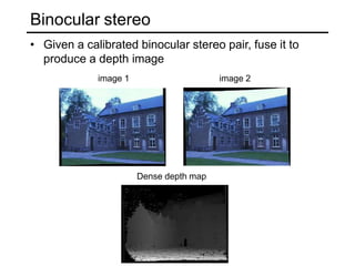
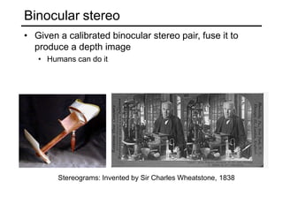
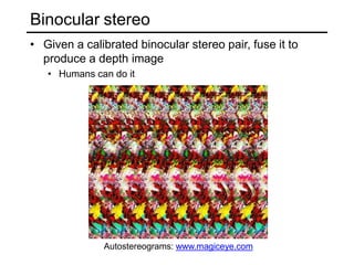
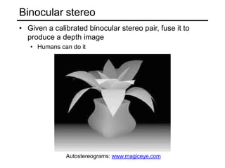
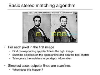
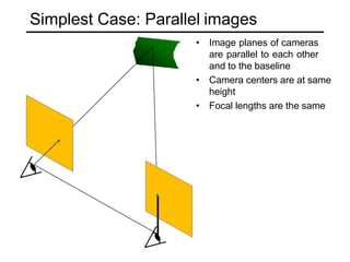
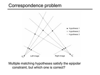
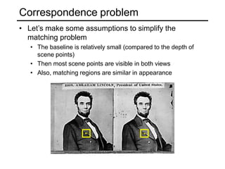
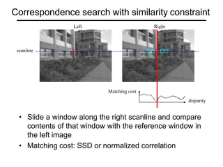
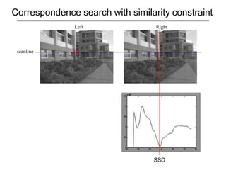
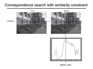
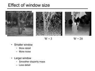
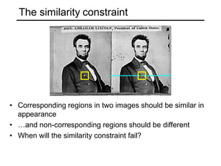
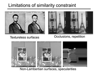
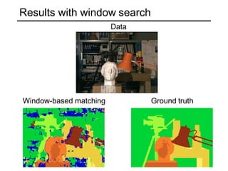
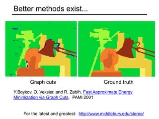
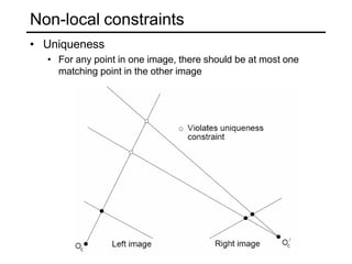
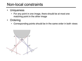
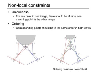
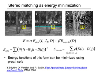
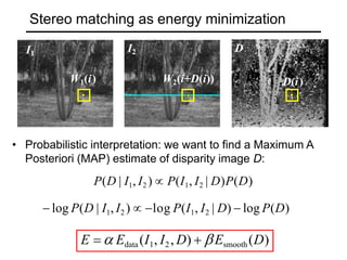
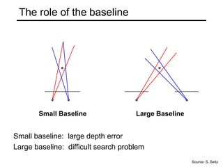
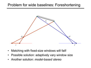
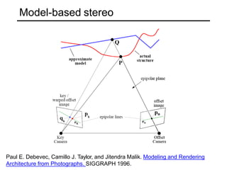
Stereo
Many slides adapted from Steve Seitz
Binocular stereo
• Given a calibrated binocular stereo pair, fuse it to
produce a depth image
image 1 image 2
Dense depth map
Binocular stereo
• Given a calibrated binocular stereo pair, fuse it to
produce a depth image
• Humans can do it
Stereograms: Invented by Sir Charles Wheatstone, 1838
Binocular stereo
• Given a calibrated binocular stereo pair, fuse it to
produce a depth image
• Humans can do it
Autostereograms: www.magiceye.com
Binocular stereo
• Given a calibrated binocular stereo pair, fuse it to
produce a depth image
• Humans can do it
Autostereograms: www.magiceye.com
Basic stereo matching algorithm
• For each pixel in the first image
• Find corresponding epipolar line in the right image
• Examine all pixels on the epipolar line and pick the best match
• Triangulate the matches to get depth information
• Simplest case: epipolar lines are scanlines
• When does this happen?
Simplest Case: Parallel images
• Image planes of cameras
are parallel to each other
and to the baseline
• Camera centers are at same
height
• Focal lengths are the same
Simplest Case: Parallel images
• Image planes of cameras
are parallel to each other
and to the baseline
• Camera centers are at same
height
• Focal lengths are the same
• Then, epipolar lines fall
along the horizontal scan
lines of the images
Depth from disparity
f
x x’
z
O Baseline
B
O’
X
f
disparity  x  x

B  f
z
Disparity is inversely proportional to depth!
Stereo image rectification
• reproject image planes onto a common
plane parallel to the line between optical centers
• pixel motion is horizontal after this transformation
• two homographies (3x3 transform), one for each
input image reprojection
 C. Loop and Z. Zhang. Computing Rectifying Homographies for
Stereo Vision. IEEE Conf. Computer Vision and Pattern Recognition,
1999.
Rectification example
Basic stereo matching algorithm
• If necessary, rectify the two stereo images to transform
epipolar lines into scanlines
• For each pixel x in the first image
• Find corresponding epipolar scanline in the right image
• Examine all pixels on the scanline and pick the best match x’
• Compute disparity x-x’ and set depth(x) = 1/(x-x’)
Correspondence problem
Multiple matching hypotheses satisfy the epipolar
constraint, but which one is correct?
Correspondence problem
• Let’s make some assumptions to simplify the
matching problem
• The baseline is relatively small (compared to the depth of
scene points)
• Then most scene points are visible in both views
• Also, matching regions are similar in appearance
Correspondence problem
• Let’s make some assumptions to simplify the
matching problem
• The baseline is relatively small (compared to the depth of
scene points)
• Then most scene points are visible in both views
• Also, matching regions are similar in appearance
Matching cost
disparity
Left Right
scanline
Correspondence search with similarity constraint
• Slide a window along the right scanline and compare
contents of that window with the reference window in
the left image
• Matching cost: SSD or normalized correlation
Left Right
scanline
Correspondence search with similarity constraint
SSD
Left Right
scanline
Correspondence search with similarity constraint
Norm. corr
Effect of window size
• Smaller window
+ More detail
– More noise
• Larger window
+ Smoother disparity maps
– Less detail
W = 3 W = 20
The similarity constraint
• Corresponding regions in two images should be similar in
appearance
• …and non-corresponding regions should be different
• When will the similarity constraint fail?
Limitations of similarity constraint
Textureless surfaces Occlusions, repetition
Non-Lambertian surfaces, specularities
Results with window search
Window-based matching Ground truth
Data
Better methods exist...
Graph cuts Ground truth
Y.Boykov, O. Veksler, and R. Zabih, Fast Approximate Energy
Minimization via Graph Cuts, PAMI 2001
For the latest and greatest: http://www.middlebury.edu/stereo/
How can we improve window-based matching?
• The similarity constraint is local (each reference
window is matched independently)
• Need to enforce non-local correspondence
constraints
Non-local constraints
• Uniqueness
• For any point in one image, there should be at most one
matching point in the other image
Non-local constraints
• Uniqueness
• For any point in one image, there should be at most one
matching point in the other image
• Ordering
• Corresponding points should be in the same order in both views
Non-local constraints
• Uniqueness
• For any point in one image, there should be at most one
matching point in the other image
• Ordering
• Corresponding points should be in the same order in both views
Ordering constraint doesn’t hold
Non-local constraints
• Uniqueness
• For any point in one image, there should be at most one
matching point in the other image
• Ordering
• Corresponding points should be in the same order in both views
• Smoothness
• We expect disparity values to change slowly (for the most part)
Scanline stereo
• Try to coherently match pixels on the entire scanline
• Different scanlines are still optimized independently
Left image Right image
“Shortest paths” for scan-line stereo
Left image
Right image
Ohta & Kanade ’85, Cox et al. ‘96
Sleft
right
S
q
Left
occlusio
n
t
Right
occlusion
s p
Can be implemented with dynamic programming
Coccl
Coccl
I
I
Ccorr
Slide credit: Y
. Boykov
Coherent stereo on 2D grid
• Scanline stereo generates streaking artifacts
• Can’t use dynamic programming to find spatially
coherent disparities/ correspondences on a 2D grid
Stereo matching as energy minimization
I1
I2 D
• Energy functions of this form can be minimized using
graph cuts
Y.Boykov, O. Veksler, and R. Zabih, Fast Approximate Energy Minimization
via Graph Cuts, PAMI 2001
W1(i) W2(i+D(i)) D(i)
E   Edata(I1, I2 , D)  Esmooth (D)
neighbors i, j
Esmooth  D(i)  D( j)
2
1 2
data 
i
W(i) W (i D(i))
E 
Stereo matching as energy minimization
I1
I2 D
W1(i) W2(i+D(i)) D(i)
• Probabilistic interpretation: we want to find a Maximum A
Posteriori (MAP) estimate of disparity image D:
P(D | I1, I2 )  P(I1, I2 | D)P(D)
 log P(D | I1, I2 )  log P(I1, I2 | D)  log P(D)
E   Edata (I1, I2, D)  Esmooth(D)
The role of the baseline
Small Baseline Large Baseline
Small baseline: large depth error
Large baseline: difficult search problem
Source: S. Seitz
Problem for wide baselines: Foreshortening
• Matching with fixed-size windows will fail!
• Possible solution: adaptively vary window size
• Another solution: model-based stereo
Model-based stereo
Paul E. Debevec, Camillo J. Taylor, and Jitendra Malik. Modeling and Rendering
Architecture from Photographs. SIGGRAPH 1996.
Model-based stereo
key image offset image
Paul E. Debevec, Camillo J. Taylor, and Jitendra Malik. Modeling and Rendering
Architecture from Photographs. SIGGRAPH 1996.
Model-based stereo
key image warped offset image
displacement map
Paul E. Debevec, Camillo J. Taylor, and Jitendra Malik. Modeling and Rendering
Architecture from Photographs. SIGGRAPH 1996.
Laser scanning
Optical triangulation
• Project a single stripe of laser light
• Scan it across the surface of the object
• This is a very precise version of structured light scanning
CCD
Laser
Object
Direction of travel
Laser sheet
CCD image plane
Cylindrical lens
Digital Michelangelo Project
http://graphics.stanford.edu/projects/mich/
Source: S. Seitz
Laser scanned models
The Digital Michelangelo Project, Levoy et al.
Source: S. Seitz
Laser scanned models
The Digital Michelangelo Project, Levoy et al.
Source: S. Seitz
Laser scanned models
The Digital Michelangelo Project, Levoy et al.
Source: S. Seitz
Laser scanned models
The Digital Michelangelo Project, Levoy et al.
Source: S. Seitz
1.0 mm resolution (56 million triangles)
Aligning range images
• A single range scan is not sufficient to describe a
complex surface
• Need techniques to register multiple range images
B. Curless and M. Levoy, A Volumetric Method for Building Complex Models from
Range Images, SIGGRAPH 1996
Aligning range images
• A single range scan is not sufficient to describe a
complex surface
• Need techniques to register multiple range images
… which brings us to multi-view stereo

Lec13 stereo converted

  • 1.
  • 2.
    Binocular stereo • Givena calibrated binocular stereo pair, fuse it to produce a depth image image 1 image 2 Dense depth map
  • 3.
    Binocular stereo • Givena calibrated binocular stereo pair, fuse it to produce a depth image • Humans can do it Stereograms: Invented by Sir Charles Wheatstone, 1838
  • 4.
    Binocular stereo • Givena calibrated binocular stereo pair, fuse it to produce a depth image • Humans can do it Autostereograms: www.magiceye.com
  • 5.
    Binocular stereo • Givena calibrated binocular stereo pair, fuse it to produce a depth image • Humans can do it Autostereograms: www.magiceye.com
  • 6.
    Basic stereo matchingalgorithm • For each pixel in the first image • Find corresponding epipolar line in the right image • Examine all pixels on the epipolar line and pick the best match • Triangulate the matches to get depth information • Simplest case: epipolar lines are scanlines • When does this happen?
  • 7.
    Simplest Case: Parallelimages • Image planes of cameras are parallel to each other and to the baseline • Camera centers are at same height • Focal lengths are the same
  • 8.
    Simplest Case: Parallelimages • Image planes of cameras are parallel to each other and to the baseline • Camera centers are at same height • Focal lengths are the same • Then, epipolar lines fall along the horizontal scan lines of the images
  • 11.
    Depth from disparity f xx’ z O Baseline B O’ X f disparity  x  x  B  f z Disparity is inversely proportional to depth!
  • 12.
  • 13.
    Stereo image rectification •reproject image planes onto a common plane parallel to the line between optical centers • pixel motion is horizontal after this transformation • two homographies (3x3 transform), one for each input image reprojection  C. Loop and Z. Zhang. Computing Rectifying Homographies for Stereo Vision. IEEE Conf. Computer Vision and Pattern Recognition, 1999.
  • 14.
  • 15.
    Basic stereo matchingalgorithm • If necessary, rectify the two stereo images to transform epipolar lines into scanlines • For each pixel x in the first image • Find corresponding epipolar scanline in the right image • Examine all pixels on the scanline and pick the best match x’ • Compute disparity x-x’ and set depth(x) = 1/(x-x’)
  • 16.
    Correspondence problem Multiple matchinghypotheses satisfy the epipolar constraint, but which one is correct?
  • 17.
    Correspondence problem • Let’smake some assumptions to simplify the matching problem • The baseline is relatively small (compared to the depth of scene points) • Then most scene points are visible in both views • Also, matching regions are similar in appearance
  • 18.
    Correspondence problem • Let’smake some assumptions to simplify the matching problem • The baseline is relatively small (compared to the depth of scene points) • Then most scene points are visible in both views • Also, matching regions are similar in appearance
  • 19.
    Matching cost disparity Left Right scanline Correspondencesearch with similarity constraint • Slide a window along the right scanline and compare contents of that window with the reference window in the left image • Matching cost: SSD or normalized correlation
  • 20.
    Left Right scanline Correspondence searchwith similarity constraint SSD
  • 21.
    Left Right scanline Correspondence searchwith similarity constraint Norm. corr
  • 22.
    Effect of windowsize • Smaller window + More detail – More noise • Larger window + Smoother disparity maps – Less detail W = 3 W = 20
  • 23.
    The similarity constraint •Corresponding regions in two images should be similar in appearance • …and non-corresponding regions should be different • When will the similarity constraint fail?
  • 24.
    Limitations of similarityconstraint Textureless surfaces Occlusions, repetition Non-Lambertian surfaces, specularities
  • 25.
    Results with windowsearch Window-based matching Ground truth Data
  • 26.
    Better methods exist... Graphcuts Ground truth Y.Boykov, O. Veksler, and R. Zabih, Fast Approximate Energy Minimization via Graph Cuts, PAMI 2001 For the latest and greatest: http://www.middlebury.edu/stereo/
  • 27.
    How can weimprove window-based matching? • The similarity constraint is local (each reference window is matched independently) • Need to enforce non-local correspondence constraints
  • 28.
    Non-local constraints • Uniqueness •For any point in one image, there should be at most one matching point in the other image
  • 29.
    Non-local constraints • Uniqueness •For any point in one image, there should be at most one matching point in the other image • Ordering • Corresponding points should be in the same order in both views
  • 30.
    Non-local constraints • Uniqueness •For any point in one image, there should be at most one matching point in the other image • Ordering • Corresponding points should be in the same order in both views Ordering constraint doesn’t hold
  • 31.
    Non-local constraints • Uniqueness •For any point in one image, there should be at most one matching point in the other image • Ordering • Corresponding points should be in the same order in both views • Smoothness • We expect disparity values to change slowly (for the most part)
  • 32.
    Scanline stereo • Tryto coherently match pixels on the entire scanline • Different scanlines are still optimized independently Left image Right image
  • 33.
    “Shortest paths” forscan-line stereo Left image Right image Ohta & Kanade ’85, Cox et al. ‘96 Sleft right S q Left occlusio n t Right occlusion s p Can be implemented with dynamic programming Coccl Coccl I I Ccorr Slide credit: Y . Boykov
  • 34.
    Coherent stereo on2D grid • Scanline stereo generates streaking artifacts • Can’t use dynamic programming to find spatially coherent disparities/ correspondences on a 2D grid
  • 35.
    Stereo matching asenergy minimization I1 I2 D • Energy functions of this form can be minimized using graph cuts Y.Boykov, O. Veksler, and R. Zabih, Fast Approximate Energy Minimization via Graph Cuts, PAMI 2001 W1(i) W2(i+D(i)) D(i) E   Edata(I1, I2 , D)  Esmooth (D) neighbors i, j Esmooth  D(i)  D( j) 2 1 2 data  i W(i) W (i D(i)) E 
  • 36.
    Stereo matching asenergy minimization I1 I2 D W1(i) W2(i+D(i)) D(i) • Probabilistic interpretation: we want to find a Maximum A Posteriori (MAP) estimate of disparity image D: P(D | I1, I2 )  P(I1, I2 | D)P(D)  log P(D | I1, I2 )  log P(I1, I2 | D)  log P(D) E   Edata (I1, I2, D)  Esmooth(D)
  • 37.
    The role ofthe baseline Small Baseline Large Baseline Small baseline: large depth error Large baseline: difficult search problem Source: S. Seitz
  • 38.
    Problem for widebaselines: Foreshortening • Matching with fixed-size windows will fail! • Possible solution: adaptively vary window size • Another solution: model-based stereo
  • 39.
    Model-based stereo Paul E.Debevec, Camillo J. Taylor, and Jitendra Malik. Modeling and Rendering Architecture from Photographs. SIGGRAPH 1996.
  • 40.
    Model-based stereo key imageoffset image Paul E. Debevec, Camillo J. Taylor, and Jitendra Malik. Modeling and Rendering Architecture from Photographs. SIGGRAPH 1996.
  • 41.
    Model-based stereo key imagewarped offset image displacement map Paul E. Debevec, Camillo J. Taylor, and Jitendra Malik. Modeling and Rendering Architecture from Photographs. SIGGRAPH 1996.
  • 42.
    Laser scanning Optical triangulation •Project a single stripe of laser light • Scan it across the surface of the object • This is a very precise version of structured light scanning CCD Laser Object Direction of travel Laser sheet CCD image plane Cylindrical lens Digital Michelangelo Project http://graphics.stanford.edu/projects/mich/ Source: S. Seitz
  • 43.
    Laser scanned models TheDigital Michelangelo Project, Levoy et al. Source: S. Seitz
  • 44.
    Laser scanned models TheDigital Michelangelo Project, Levoy et al. Source: S. Seitz
  • 45.
    Laser scanned models TheDigital Michelangelo Project, Levoy et al. Source: S. Seitz
  • 46.
    Laser scanned models TheDigital Michelangelo Project, Levoy et al. Source: S. Seitz 1.0 mm resolution (56 million triangles)
  • 47.
    Aligning range images •A single range scan is not sufficient to describe a complex surface • Need techniques to register multiple range images B. Curless and M. Levoy, A Volumetric Method for Building Complex Models from Range Images, SIGGRAPH 1996
  • 48.
    Aligning range images •A single range scan is not sufficient to describe a complex surface • Need techniques to register multiple range images … which brings us to multi-view stereo