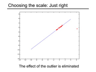
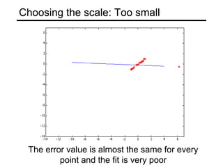
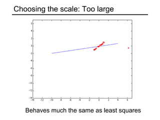
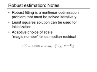
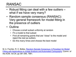
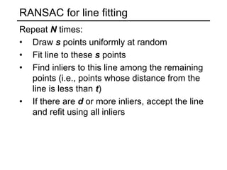
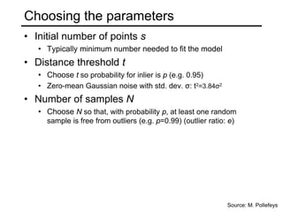
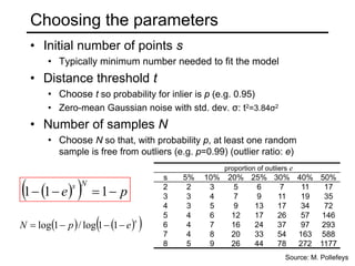
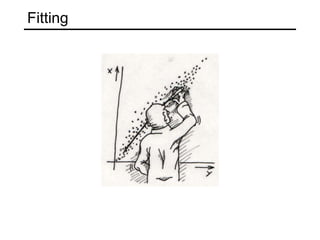
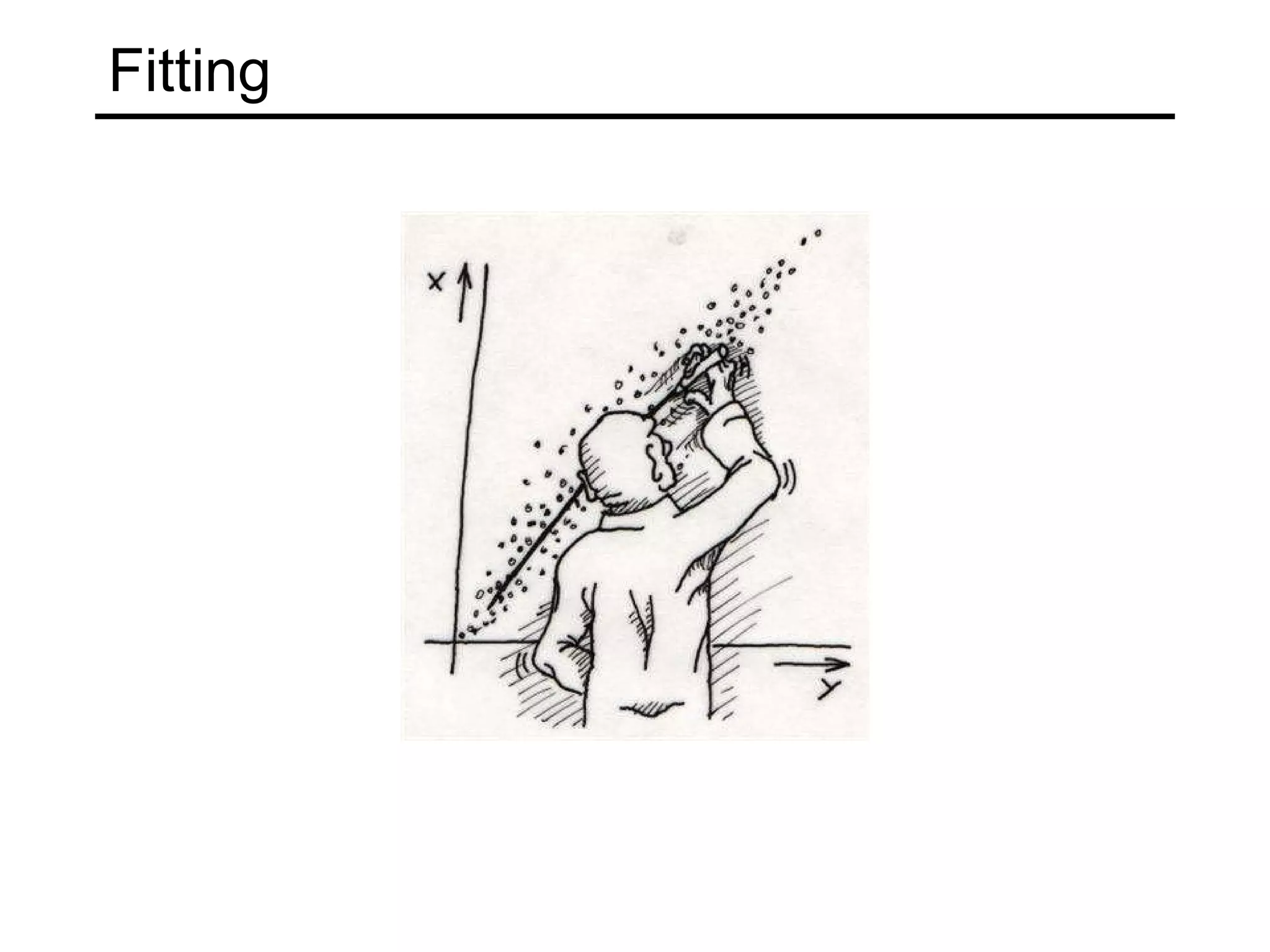
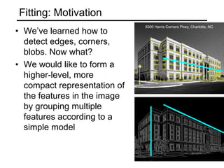
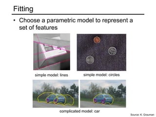
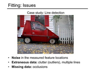
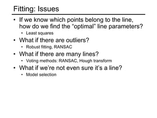
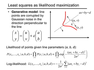
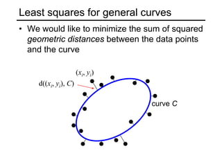
This document discusses techniques for fitting parametric models to sets of image features. It begins by introducing the concept of fitting, where a simple parametric model (like a line or circle) is used to represent multiple detected features. It describes how fitting involves choosing the best model, assigning features to model instances, and determining the number of instances. The document then discusses specific issues that arise, such as noise, outliers, missing data, and model selection. It presents techniques for line fitting, including least squares, total least squares, and robust methods like RANSAC. It also discusses fitting general curves and conics using least squares approaches.

1. Fitting

2. Fitting: Motivation
• We’ve learned how to
detect edges, corners,
blobs. Now what?
• We would like to form a
higher-level, more
compact representation of
the features in the image
by grouping multiple
features according to a
simple model
9300 Harris Corners Pkwy, Charlotte, NC

3. Source: K. Grauman
Fitting
• Choose a parametric model to represent a
set of features
simple model: lines simple model: circles
complicated model: car

4. Fitting
• Choose a parametric model to represent a
set of features
• Membership criterion is not local
• Can’t tell whether a point belongs to a given model just by
looking at that point
• Three main questions:
• What model represents this set of features best?
• Which of several model instances gets which feature?
• How many model instances are there?
• Computational complexity is important
• It is infeasible to examine every possible set of parameters
and every possible combination of features

5. Fitting: Issues
• Noise in the measured feature locations
• Extraneous data: clutter (outliers), multiple lines
• Missing data: occlusions
Case study: Line detection

6. Fitting: Issues
• If we know which points belong to the line,
how do we find the “optimal” line parameters?
• Least squares
• What if there are outliers?
• Robust fitting, RANSAC
• What if there are many lines?
• Voting methods: RANSAC, Hough transform
• What if we’re not even sure it’s a line?
• Model selection

7. Least squares line fitting
Data: (x1, y1), …, (xn, yn)
Line equation: yi = m xi + b
Find (m, b) to minimize
∑=
−
−
=
n
i i
i b
x
m
y
E 1
2
)
(
(xi, yi)
y=mx+b

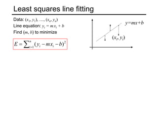
8. Least squares line fitting
Data: (x1, y1), …, (xn, yn)
Line equation: yi = m xi + b
Find (m, b) to minimize
0
2
2 =
−
= Y
X
XB
X
dB
dE T
T
[ ]
)
(
)
(
)
(
2
)
(
)
(
1
1
1
2
2
1
1
1
2
XB
XB
Y
XB
Y
Y
XB
Y
XB
Y
XB
Y
b
m
x
x
y
y
b
m
x
y
E
T
T
T
T
n
n
n
i i
i
+
−
=
−
−
=
−
=
⎥
⎦
⎤
⎢
⎣
⎡
⎥
⎥
⎥
⎦
⎤
⎢
⎢
⎢
⎣
⎡
−
⎥
⎥
⎥
⎦
⎤
⎢
⎢
⎢
⎣
⎡
=
⎟
⎟
⎠
⎞
⎜
⎜
⎝
⎛
⎥
⎦
⎤
⎢
⎣
⎡
−
= ∑=
M
M
M
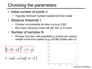
Normal equations: least squares solution to
XB=Y
∑=
−
−
=
n
i i
i b
x
m
y
E 1
2
)
(
(xi, yi)
y=mx+b
Y
X
XB
X T
T
=

9. Problem with “vertical” least squares
• Not rotation-invariant
• Fails completely for vertical lines

10. Total least squares
Distance between point (xn, yn) and
line ax+by=d (a2+b2=1): |ax + by – d|
Find (a, b, d) to minimize the sum of
squared perpendicular distances ∑=
−
+
=
n
i i
i d
y
b
x
a
E 1
2
)
( (xi, yi)
ax+by=d
∑=
−
+
=
n
i i
i d
y
b
x
a
E 1
2
)
(
Unit normal:
N=(a, b)

11. Total least squares
Distance between point (xn, yn) and
line ax+by=d (a2+b2=1): |ax + by – d|
Find (a, b, d) to minimize the sum of
squared perpendicular distances ∑=
−
+
=
n
i i
i d
y
b
x
a
E 1
2
)
( (xi, yi)
ax+by=d
∑=
−
+
=
n
i i
i d
y
b
x
a
E 1
2
)
(
Unit normal:
N=(a, b)
0
)
(
2
1
=
−
+
−
=
∂
∂
∑=
n
i i
i d
y
b
x
a
d
E
y
b
x
a
x
n
b
x
n
a
d
n
i i
n
i i +
=
+
= ∑
∑ =
= 1
1
)
(
)
(
))
(
)
(
(
2
1
1
1
2
UN
UN
b
a
y
y
x
x
y
y
x
x
y
y
b
x
x
a
E T
n
n
n
i i
i =
⎥
⎦
⎤
⎢
⎣
⎡
⎥
⎥
⎥
⎦
⎤
⎢
⎢
⎢
⎣
⎡
−
−
−
−
=
−
+
−
= ∑=
M
M
0
)
(
2 =
= N
U
U
dN
dE T
Solution to (UTU)N = 0, subject to ||N||2 = 1: eigenvector of UTU
associated with the smallest eigenvalue (least squares solution
to homogeneous linear system UN = 0)

12. Total least squares
⎥
⎥
⎥
⎦
⎤
⎢
⎢
⎢
⎣
⎡
−
−
−
−
=
y
y
x
x
y
y
x
x
U
n
n
M
M
1
1
⎥
⎥
⎥
⎥
⎦
⎤
⎢
⎢
⎢
⎢
⎣
⎡
−
−
−
−
−
−
=
∑
∑
∑
∑
=
=
=
=
n
i
i
n
i
i
i
n
i
i
i
n
i
i
T
y
y
y
y
x
x
y
y
x
x
x
x
U
U
1
2
1
1
1
2
)
(
)
)(
(
)
)(
(
)
(
second moment matrix

13. Total least squares
⎥
⎥
⎥
⎦
⎤
⎢
⎢
⎢
⎣
⎡
−
−
−
−
=
y
y
x
x
y
y
x
x
U
n
n
M
M
1
1
⎥
⎥
⎥
⎥
⎦
⎤
⎢
⎢
⎢
⎢
⎣
⎡
−
−
−
−
−
−
=
∑
∑
∑
∑
=
=
=
=
n
i
i
n
i
i
i
n
i
i
i
n
i
i
T
y
y
y
y
x
x
y
y
x
x
x
x
U
U
1
2
1
1
1
2
)
(
)
)(
(
)
)(
(
)
(
)
,
( y
x
N = (a, b)
second moment matrix
)
,
( y
y
x
x i
i −
−

14. Least squares as likelihood maximization
• Generative model: line
points are corrupted by
Gaussian noise in the
direction perpendicular to
the line
⎟
⎟
⎠
⎞
⎜
⎜
⎝
⎛
+
⎟
⎟
⎠
⎞
⎜
⎜
⎝
⎛
=
⎟
⎟
⎠
⎞
⎜
⎜
⎝
⎛
b
a
v
u
y
x
ε
(x, y)
ax+by=d
(u, v)
ε
point
on the
line
noise:
zero-mean
Gaussian with
std. dev. σ
normal
direction

15. Least squares as likelihood maximization
• Generative model: line
points are corrupted by
Gaussian noise in the
direction perpendicular to
the line
⎟
⎟
⎠
⎞
⎜
⎜
⎝
⎛
+
⎟
⎟
⎠
⎞
⎜
⎜
⎝
⎛
=
⎟
⎟
⎠
⎞
⎜
⎜
⎝
⎛
b
a
v
u
y
x
ε
(x, y)
(u, v)
ε
∏
∏ =
=
⎟
⎟
⎠
⎞
⎜
⎜
⎝
⎛ −
+
−
∝
=
n
i
i
i
n
i
i
n
d
by
ax
d
b
a
x
P
d
b
a
x
x
P
1
2
2
1
1
2
)
(
exp
)
,
,
|
(
)
,
,
|
,
,
(
σ
K
Likelihood of points given line parameters (a, b, d):
∑
=
−
+
−
=
n
i
i
i
n d
by
ax
d
b
a
x
x
L
1
2
2
1 )
(
2
1
)
,
,
|
,
,
(
σ
K
Log-likelihood:
ax+by=d

16. Least squares for general curves
• We would like to minimize the sum of squared
geometric distances between the data points
and the curve
(xi, yi)
d((xi, yi), C)
curve C

17. Least squares for conics
• Equation of a general conic:
C(a, x) = a · x = ax2 + bxy + cy2 + dx + ey + f = 0,
a = [a, b, c, d, e, f],
x = [x2, xy, y2, x, y, 1]
• Minimizing the geometric distance is non-linear even for
a conic
• Algebraic distance: C(a, x)
• Algebraic distance minimization by linear least squares:
0
1
1
1
2
2
2
2
2
2
2
2
2
2
1
1
2
1
1
1
2
1
=
⎥
⎥
⎥
⎥
⎥
⎥
⎥
⎥
⎦
⎤
⎢
⎢
⎢
⎢
⎢
⎢
⎢
⎢
⎣
⎡
⎥
⎥
⎥
⎥
⎥
⎦
⎤
⎢
⎢
⎢
⎢
⎢
⎣
⎡
f
e
d
c
b
a
y
x
y
y
x
x
y
x
y
y
x
x
y
x
y
y
x
x
n
n
n
n
n
n
M
O
M

18. Least squares for conics
• Least squares system: Da = 0
• Need constraint on a to prevent trivial solution
• Discriminant: b2 – 4ac
• Negative: ellipse
• Zero: parabola
• Positive: hyperbola
• Minimizing squared algebraic distance subject to
constraints leads to a generalized eigenvalue
problem
• Many variations possible
• For more information:
• A. Fitzgibbon, M. Pilu, and R. Fisher, Direct least-squares fitting
of ellipses, IEEE Transactions on Pattern Analysis and Machine
Intelligence, 21(5), 476--480, May 1999

19. Least squares: Robustness to noise
Least squares fit to the red points:

20. Least squares: Robustness to noise
Least squares fit with an outlier:
Problem: squared error heavily penalizes outliers

21. Robust estimators
• General approach: minimize
ri (xi, θ) – residual of ith point w.r.t. model parameters θ
ρ – robust function with scale parameter σ
( )
( )
σ
θ
ρ ;
,
i
i
i
x
r
∑
The robust function
ρ behaves like
squared distance for
small values of the
residual u but
saturates for larger
values of u

22. Choosing the scale: Just right
The effect of the outlier is eliminated

23. The error value is almost the same for every
point and the fit is very poor
Choosing the scale: Too small

24. Choosing the scale: Too large
Behaves much the same as least squares

25. Robust estimation: Notes
• Robust fitting is a nonlinear optimization
problem that must be solved iteratively
• Least squares solution can be used for
initialization
• Adaptive choice of scale:
“magic number” times median residual

26. RANSAC
• Robust fitting can deal with a few outliers –
what if we have very many?
• Random sample consensus (RANSAC):
Very general framework for model fitting in
the presence of outliers
• Outline
• Choose a small subset uniformly at random
• Fit a model to that subset
• Find all remaining points that are “close” to the model and
reject the rest as outliers
• Do this many times and choose the best model
M. A. Fischler, R. C. Bolles. Random Sample Consensus: A Paradigm for Model
Fitting with Applications to Image Analysis and Automated Cartography. Comm. of
the ACM, Vol 24, pp 381-395, 1981.

27. RANSAC for line fitting
Repeat N times:
• Draw s points uniformly at random
• Fit line to these s points
• Find inliers to this line among the remaining
points (i.e., points whose distance from the
line is less than t)
• If there are d or more inliers, accept the line
and refit using all inliers

28. Choosing the parameters
• Initial number of points s
• Typically minimum number needed to fit the model
• Distance threshold t
• Choose t so probability for inlier is p (e.g. 0.95)
• Zero-mean Gaussian noise with std. dev. σ: t2=3.84σ2
• Number of samples N
• Choose N so that, with probability p, at least one random
sample is free from outliers (e.g. p=0.99) (outlier ratio: e)
Source: M. Pollefeys

29. Choosing the parameters
• Initial number of points s
• Typically minimum number needed to fit the model
• Distance threshold t
• Choose t so probability for inlier is p (e.g. 0.95)
• Zero-mean Gaussian noise with std. dev. σ: t2=3.84σ2
• Number of samples N
• Choose N so that, with probability p, at least one random
sample is free from outliers (e.g. p=0.99) (outlier ratio: e)
( ) ( )
( )
s
e
p
N −
−
−
= 1
1
log
/
1
log
( )
( ) p
e
N
s
−
=
−
− 1
1
1
proportion of outliers e
s 5% 10% 20% 25% 30% 40% 50%
2 2 3 5 6 7 11 17
3 3 4 7 9 11 19 35
4 3 5 9 13 17 34 72
5 4 6 12 17 26 57 146
6 4 7 16 24 37 97 293
7 4 8 20 33 54 163 588
8 5 9 26 44 78 272 1177
Source: M. Pollefeys

30. Choosing the parameters
• Initial number of points s
• Typically minimum number needed to fit the model
• Distance threshold t
• Choose t so probability for inlier is p (e.g. 0.95)
• Zero-mean Gaussian noise with std. dev. σ: t2=3.84σ2
• Number of samples N
• Choose N so that, with probability p, at least one random
sample is free from outliers (e.g. p=0.99) (outlier ratio: e)
( )
( ) p
e
N
s
−
=
−
− 1
1
1
Source: M. Pollefeys
( ) ( )
( )
s
e
p
N −
−
−
= 1
1
log
/
1
log

31. Choosing the parameters
• Initial number of points s
• Typically minimum number needed to fit the model
• Distance threshold t
• Choose t so probability for inlier is p (e.g. 0.95)
• Zero-mean Gaussian noise with std. dev. σ: t2=3.84σ2
• Number of samples N
• Choose N so that, with probability p, at least one random
sample is free from outliers (e.g. p=0.99) (outlier ratio: e)
• Consensus set size d
• Should match expected inlier ratio
Source: M. Pollefeys

32. Adaptively determining the number of samples
• Inlier ratio e is often unknown a priori, so pick
worst case, e.g. 50%, and adapt if more
inliers are found, e.g. 80% would yield e=0.2
• Adaptive procedure:
• N=∞, sample_count =0
• While N >sample_count
– Choose a sample and count the number of inliers
– Set e = 1 – (number of inliers)/(total number of points)
– Recompute N from e:
– Increment the sample_count by 1
( ) ( )
( )
s
e
p
N −
−
−
= 1
1
log
/
1
log
Source: M. Pollefeys

33. RANSAC pros and cons
• Pros
• Simple and general
• Applicable to many different problems
• Often works well in practice
• Cons
• Lots of parameters to tune
• Can’t always get a good initialization of the model based on
the minimum number of samples
• Sometimes too many iterations are required
• Can fail for extremely low inlier ratios
• We can often do better than brute-force sampling