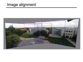
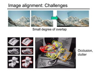
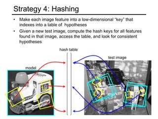
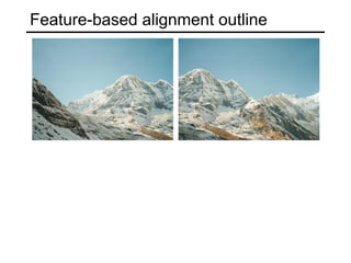
- Image alignment is used for tasks like panorama stitching and object recognition. It involves finding the transformation between two images. - There are two main approaches: direct/pixel-based alignment searches for pixel agreement, and feature-based alignment searches for agreement between extracted features and can be verified using pixel alignment. - Feature-based alignment first extracts features, computes putative matches between features, then hypothesizes and verifies transformations between small groups of matches.

1. Image alignment

2. Image alignment: Motivation
Panorama stitching
Recognition
of object
instances

3. Image alignment: Challenges
Small degree of overlap
Occlusion,
clutter

4. Image alignment
• Two broad approaches:
• Direct (pixel-based) alignment
– Search for alignment where most pixels agree
• Feature-based alignment
– Search for alignment where extracted features agree
– Can be verified using pixel-based alignment

5. Alignment as fitting
• Previous lectures: fitting a model to features in one image
∑
i
i M
x )
,
(
residual
Find model M that minimizes
M
xi

6. Alignment as fitting
• Previous lectures: fitting a model to features in one image
• Alignment: fitting a model to a transformation between
pairs of features (matches) in two images
∑
i
i M
x )
,
(
residual
∑ ′
i
i
i x
x
T )
),
(
(
residual
Find model M that minimizes
Find transformation T
that minimizes
M
xi
T
xi
xi
'

7. Feature-based alignment outline

8. Feature-based alignment outline
• Extract features

9. Feature-based alignment outline
• Extract features
• Compute putative matches

10. Feature-based alignment outline
• Extract features
• Compute putative matches
• Loop:
• Hypothesize transformation T (small group of putative
matches that are related by T)

11. Feature-based alignment outline
• Extract features
• Compute putative matches
• Loop:
• Hypothesize transformation T (small group of putative
matches that are related by T)
• Verify transformation (search for other matches consistent
with T)

12. Feature-based alignment outline
• Extract features
• Compute putative matches
• Loop:
• Hypothesize transformation T (small group of putative
matches that are related by T)
• Verify transformation (search for other matches consistent
with T)

13. 2D transformation models
• Similarity
(translation,
scale, rotation)
• Affine
• Projective
(homography)

14. Let’s start with affine transformations
• Simple fitting procedure (linear least squares)
• Approximates viewpoint changes for roughly planar
objects and roughly orthographic cameras
• Can be used to initialize fitting for more complex
models

15. Fitting an affine transformation
• Assume we know the correspondences, how do we
get the transformation?
)
,
( i
i y
x ′
′
)
,
( i
i y
x
⎥
⎦
⎤
⎢
⎣
⎡
+
⎥
⎦
⎤
⎢
⎣
⎡
⎥
⎦
⎤
⎢
⎣
⎡
=
⎥
⎦
⎤
⎢
⎣
⎡
′
′
2
1
4
3
2
1
t
t
y
x
m
m
m
m
y
x
i
i
i
i
⎥
⎥
⎥
⎥
⎦
⎤
⎢
⎢
⎢
⎢
⎣
⎡
′
′
=
⎥
⎥
⎥
⎥
⎥
⎥
⎥
⎥
⎦
⎤
⎢
⎢
⎢
⎢
⎢
⎢
⎢
⎢
⎣
⎡
⎥
⎥
⎥
⎥
⎦
⎤
⎢
⎢
⎢
⎢
⎣
⎡
L
L
L
L
i
i
i
i
i
i
y
x
t
t
m
m
m
m
y
x
y
x
2
1
4
3
2
1
1
0
0
0
0
1
0
0

16. Fitting an affine transformation
• Linear system with six unknowns
• Each match gives us two linearly independent
equations: need at least three to solve for the
transformation parameters
⎥
⎥
⎥
⎥
⎦
⎤
⎢
⎢
⎢
⎢
⎣
⎡
′
′
=
⎥
⎥
⎥
⎥
⎥
⎥
⎥
⎥
⎦
⎤
⎢
⎢
⎢
⎢
⎢
⎢
⎢
⎢
⎣
⎡
⎥
⎥
⎥
⎥
⎦
⎤
⎢
⎢
⎢
⎢
⎣
⎡
L
L
L
L
i
i
i
i
i
i
y
x
t
t
m
m
m
m
y
x
y
x
2
1
4
3
2
1
1
0
0
0
0
1
0
0

17. What if we don’t know the correspondences?
?

18. What if we don’t know the correspondences?
• Need to compare feature descriptors of local patches
surrounding interest points
( ) ( )
=
?
feature
descriptor
feature
descriptor
?

19. Feature descriptors
• Assuming the patches are already normalized (i.e.,
the local effect of the geometric transformation is
factored out), how do we compute their similarity?
• Want invariance to intensity changes, noise,
perceptually insignificant changes of the pixel pattern

20. • Simplest descriptor: vector of raw intensity values
• How to compare two such vectors?
• Sum of squared differences (SSD)
– Not invariant to intensity change
• Normalized correlation
– Invariant to affine intensity change
Feature descriptors
( )
∑ −
=
i
i
i v
u
v
u
2
)
,
SSD(
⎟
⎟
⎠
⎞
⎜
⎜
⎝
⎛
−
⎟
⎟
⎠
⎞
⎜
⎜
⎝
⎛
−
−
−
=
∑
∑
∑
j
j
j
j
i i
i
v
v
u
u
v
v
u
u
v
u
2
2
)
(
)
(
)
)(
(
)
,
(
ρ

21. Feature descriptors
• Disadvantage of patches as descriptors:
• Small shifts can affect matching score a lot
• Solution: histograms
0 2 π

22. • Descriptor computation:
• Divide patch into 4x4 sub-patches
• Compute histogram of gradient orientations (8 reference
angles) inside each sub-patch
• Resulting descriptor: 4x4x8 = 128 dimensions
Feature descriptors: SIFT
David G. Lowe. "Distinctive image features from scale-invariant keypoints.” IJCV 60
(2), pp. 91-110, 2004.

23. • Descriptor computation:
• Divide patch into 4x4 sub-patches
• Compute histogram of gradient orientations (8 reference
angles) inside each sub-patch
• Resulting descriptor: 4x4x8 = 128 dimensions
• Advantage over raw vectors of pixel values
• Gradients less sensitive to illumination change
• “Subdivide and disorder” strategy achieves robustness to
small shifts, but still preserves some spatial information
Feature descriptors: SIFT
David G. Lowe. "Distinctive image features from scale-invariant keypoints.” IJCV 60
(2), pp. 91-110, 2004.

24. Feature matching
?
• Generating putative matches: for each patch in one
image, find a short list of patches in the other image
that could match it based solely on appearance

25. Feature matching
• Generating putative matches: for each patch in one
image, find a short list of patches in the other image
that could match it based solely on appearance
• Exhaustive search
– For each feature in one image, compute the distance to all
features in the other image and find the “closest” ones
(threshold or fixed number of top matches)
• Fast approximate nearest neighbor search
– Hierarchical spatial data structures (kd-trees, vocabulary trees)
– Hashing

26. Feature space outlier rejection
• How can we tell which putative matches are more
reliable?
• Heuristic: compare distance of nearest neighbor to
that of second nearest neighbor
• Ratio will be high for features that are not distinctive
• Threshold of 0.8 provides good separation
David G. Lowe. "Distinctive image features from scale-invariant keypoints.” IJCV 60
(2), pp. 91-110, 2004.

27. Reading
David G. Lowe. "Distinctive image features from scale-
invariant keypoints.” IJCV 60 (2), pp. 91-110, 2004.

28. Dealing with outliers
• The set of putative matches contains a very high
percentage of outliers
• Heuristics for feature-space outlier rejection
• Geometric fitting strategies:
• RANSAC
• Incremental alignment
• Hough transform
• Hashing

29. Strategy 1: RANSAC
RANSAC loop:
1. Randomly select a seed group of matches
2. Compute transformation from seed group
3. Find inliers to this transformation
4. If the number of inliers is sufficiently large, re-compute
least-squares estimate of transformation on all of the
inliers
Keep the transformation with the largest number of inliers

30. RANSAC example: Translation
Putative matches

31. RANSAC example: Translation
Select one match, count inliers

32. RANSAC example: Translation
Select one match, count inliers

33. RANSAC example: Translation
Select translation with the most inliers

34. Problem with RANSAC
• In many practical situations, the percentage of
outliers (incorrect putative matches) is often very high
(90% or above)
• Alternative strategy: restrict search space by using
strong locality constraints on seed groups and inliers
• Incremental alignment

35. Strategy 2: Incremental alignment
• Take advantage of strong locality constraints: only
pick close-by matches to start with, and gradually add
more matches in the same neighborhood
S. Lazebnik, C. Schmid and J. Ponce, “Semi-local affine parts for object
recognition,” BMVC 2004.

36. Strategy 2: Incremental alignment
• Take advantage of strong locality constraints: only
pick close-by matches to start with, and gradually add
more matches in the same neighborhood

37. Strategy 2: Incremental alignment
• Take advantage of strong locality constraints: only
pick close-by matches to start with, and gradually add
more matches in the same neighborhood

38. Strategy 2: Incremental alignment
• Take advantage of strong locality constraints: only
pick close-by matches to start with, and gradually add
more matches in the same neighborhood

39. A
Strategy 2: Incremental alignment
• Take advantage of strong locality constraints: only
pick close-by matches to start with, and gradually add
more matches in the same neighborhood

40. Strategy 3: Hough transform
• Recall: Generalized Hough transform
B. Leibe, A. Leonardis, and B. Schiele, Combined Object Categorization and Segmentation with
an Implicit Shape Model, ECCV Workshop on Statistical Learning in Computer Vision 2004
model
visual codeword with
displacement vectors
test image

41. Strategy 3: Hough transform
• Suppose our features are adapted to scale and rotation
• Then a single feature match provides an alignment hypothesis
(translation, scale, orientation)
David G. Lowe. "Distinctive image features from scale-invariant keypoints.”
IJCV 60 (2), pp. 91-110, 2004.
model

42. Strategy 3: Hough transform
• Suppose our features are adapted to scale and rotation
• Then a single feature match provides an alignment hypothesis
(translation, scale, orientation)
• Of course, a hypothesis obtained from a single match is unreliable
• Solution: let each match vote for its hypothesis in a Hough space
with very coarse bins
David G. Lowe. "Distinctive image features from scale-invariant keypoints.”
IJCV 60 (2), pp. 91-110, 2004.
model

43. Hough transform details (D. Lowe’s system)
• Training phase: For each model feature, record 2D
location, scale, and orientation of model (relative to
normalized feature frame)
• Test phase: Let each match between a test and a
model feature vote in a 4D Hough space
• Use broad bin sizes of 30 degrees for orientation, a factor of
2 for scale, and 0.25 times image size for location
• Vote for two closest bins in each dimension
• Find all bins with at least three votes and perform
geometric verification
• Estimate least squares affine transformation
• Use stricter thresholds on transformation residual
• Search for additional features that agree with the alignment
David G. Lowe. "Distinctive image features from scale-invariant keypoints.”
IJCV 60 (2), pp. 91-110, 2004.

44. Strategy 4: Hashing
• Make each image feature into a low-dimensional “key” that
indexes into a table of hypotheses
model
hash table

45. Strategy 4: Hashing
• Make each image feature into a low-dimensional “key” that
indexes into a table of hypotheses
• Given a new test image, compute the hash keys for all features
found in that image, access the table, and look for consistent
hypotheses
model
hash table
test image

46. Strategy 4: Hashing
• Make each image feature into a low-dimensional “key” that
indexes into a table of hypotheses
• Given a new test image, compute the hash keys for all features
found in that image, access the table, and look for consistent
hypotheses
• This can even work when we don’t have any feature descriptors:
we can take n-tuples of neighboring features and compute
invariant hash codes from their geometric configurations
A
B
C
D

47. Application: Searching the sky
http://www.astrometry.net/

48. Beyond affine transformations
• Homography: plane projective transformation
(transformation taking a quad to another arbitrary
quad)

49. Homography
• The transformation between two views of a planar
surface
• The transformation between images from two
cameras that share the same center

50. Fitting a homography
• Recall: homogenenous coordinates
Converting to homogenenous
image coordinates
Converting from homogenenous
image coordinates

51. Fitting a homography
• Recall: homogenenous coordinates
• Equation for homography:
Converting to homogenenous
image coordinates
Converting from homogenenous
image coordinates
⎥
⎥
⎥
⎦
⎤
⎢
⎢
⎢
⎣
⎡
⎥
⎥
⎥
⎦
⎤
⎢
⎢
⎢
⎣
⎡
=
⎥
⎥
⎥
⎦
⎤
⎢
⎢
⎢
⎣
⎡
′
′
1
1 33
32
31
23
22
21
13
12
11
y
x
h
h
h
h
h
h
h
h
h
y
x
λ

52. Fitting a homography
• Equation for homography:
i
T
T
T
i
i x
h
h
h
x
H
x
⎥
⎥
⎥
⎦
⎤
⎢
⎢
⎢
⎣
⎡
=
=
′
3
2
1
λ
⎥
⎥
⎥
⎦
⎤
⎢
⎢
⎢
⎣
⎡
⎥
⎥
⎥
⎦
⎤
⎢
⎢
⎢
⎣
⎡
=
⎥
⎥
⎥
⎦
⎤
⎢
⎢
⎢
⎣
⎡
′
′
1
1 33
32
31
23
22
21
13
12
11
i
i
i
i
y
x
h
h
h
h
h
h
h
h
h
y
x
λ
0
=
×
′ i
i x
H
x
⎥
⎥
⎥
⎦
⎤
⎢
⎢
⎢
⎣
⎡
′
−
′
′
−
−
′
=
×
′
i
T
i
i
T
i
i
T
i
i
T
i
T
i
T
i
i
i
y
x
x
y
x
h
x
h
x
h
x
h
x
h
x
h
x
H
x
1
2
3
1
2
3
0
0
0
0
3
2
1
=
⎟
⎟
⎟
⎠
⎞
⎜
⎜
⎜
⎝
⎛
⎥
⎥
⎥
⎦
⎤
⎢
⎢
⎢
⎣
⎡
′
′
−
′
−
′
−
h
h
h
x
x
x
x
x
x
T
T
i
i
T
i
i
T
i
i
T
T
i
T
i
i
T
i
T
x
y
x
y
3 equations, only 2 linearly
independent
9 entries, 8 degrees of freedom
(scale is arbitrary)

53. Direct linear transform
• H has 8 degrees of freedom (9 parameters, but scale
is arbitrary)
• One match gives us two linearly independent
equations
• Four matches needed for a minimal solution (null
space of 8x9 matrix)
• More than four: homogeneous least squares
0
0
0
0
0
3
2
1
1
1
1
1
1
1
=
⎟
⎟
⎟
⎠
⎞
⎜
⎜
⎜
⎝
⎛
⎥
⎥
⎥
⎥
⎥
⎥
⎦
⎤
⎢
⎢
⎢
⎢
⎢
⎢
⎣
⎡
′
−
′
−
′
−
′
−
h
h
h
x
x
x
x
x
x
x
x
T
n
n
T
T
n
T
n
n
T
n
T
T
T
T
T
T
T
x
y
x
y
L
L
L 0
=
h
A

54. Application: Panorama stitching

55. Recognizing panoramas
M. Brown and D. Lowe, “Recognizing Panoramas,” ICCV 2003.
• Given contents of a camera memory card,
automatically figure out which pictures go together
and stitch them together into panoramas
http://www.cs.ubc.ca/~mbrown/panorama/panorama.html

56. Issues in alignment-based applications
• Choosing the geometric alignment model
• Tradeoff between “correctness” and robustness (also,
efficiency)
• Choosing the descriptor
• “Rich” imagery (natural images): high-dimensional patch-based
descriptors (e.g., SIFT)
• “Impoverished” imagery (e.g., star fields): need to create
invariant geometric descriptors from k-tuples of point-based
features
• Strategy for finding putative matches
• Small number of images, one-time computation (e.g., panorama
stitching): brute force search
• Large database of model images, frequent queries: indexing or
hashing
• Heuristics for feature-space pruning of putative matches

57. Issues in alignment-based applications
• Choosing the geometric alignment model
• Choosing the descriptor
• Strategy for finding putative matches
• Hypothesis generation strategy
• Relatively large inlier ratio: RANSAC
• Small inlier ratio: locality constraints, Hough transform
• Hypothesis verification strategy
• Size of consensus set, residual tolerance depend on inlier ratio
and expected accuracy of the model
• Possible refinement of geometric model
• Dense verification

58. Next time: Single-view geometry