Course: Machine Vision
Image Matching
Session 12
D5627 – I Gede Putra Kusuma Negara, B.Eng., PhD
Outline
• Definition
• Invariant features
• Scale Invariant Feature Transform
• Feature matching
Definition
Definition
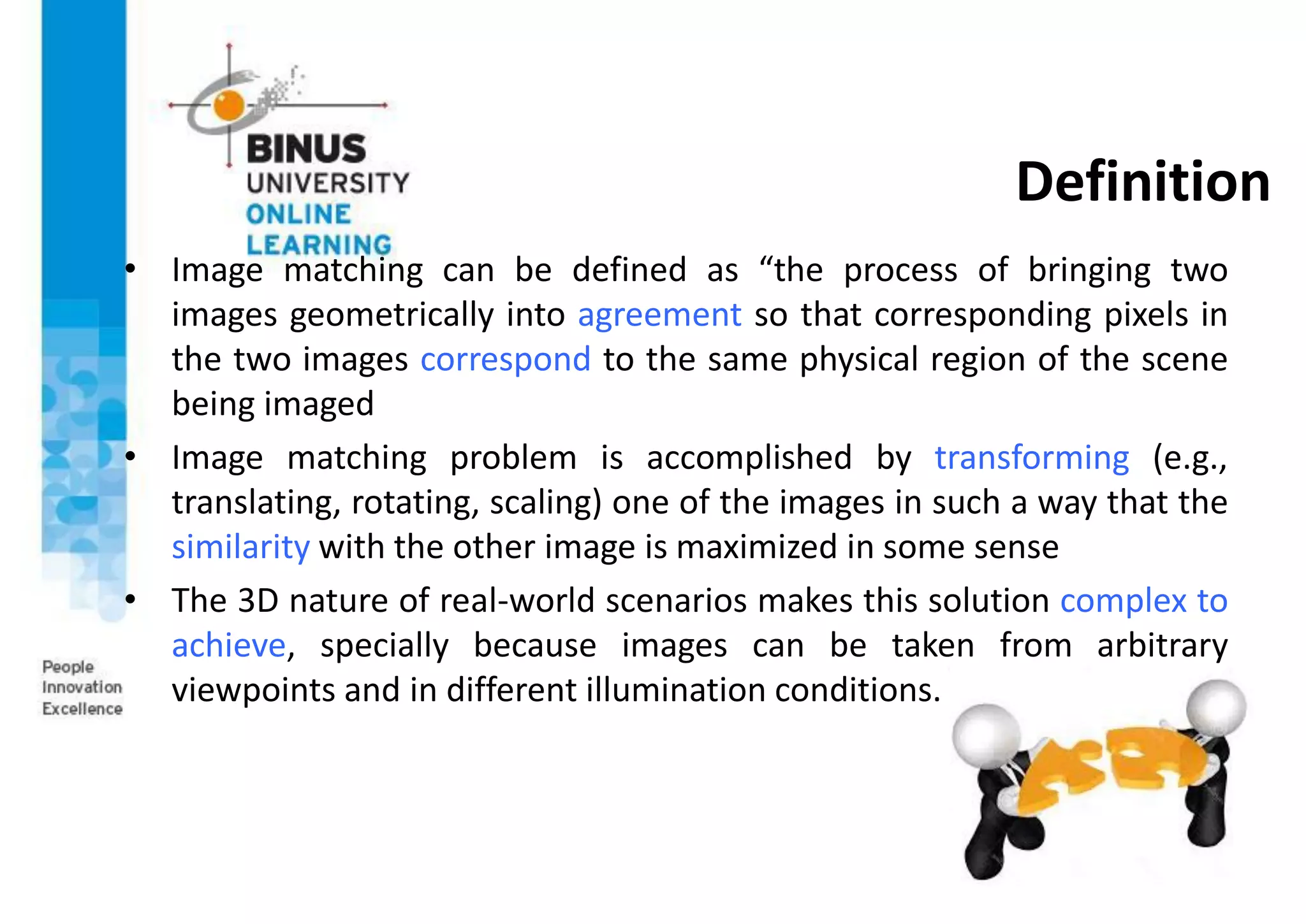
• Image matching can be defined as “the process of bringing two
images geometrically into agreement so that corresponding pixels in
the two images correspond to the same physical region of the scene
being imaged
• Image matching problem is accomplished by transforming (e.g.,
translating, rotating, scaling) one of the images in such a way that the
similarity with the other image is maximized in some sense
• The 3D nature of real-world scenarios makes this solution complex to
achieve, specially because images can be taken from arbitrary
viewpoints and in different illumination conditions.
Image Matching
• Image matching is a fundamental aspect of many problems in
computer vision, including object and scene recognition, content-
based image retrieval, stereo correspondence, motion tracking,
texture classification and video data mining.
• It is a complex problem, that remains challenging due to partial
occlusions, image deformations, and viewpoint or lighting changes
that may occur across different images
Image Matching (example)
by Diva Sian
by swashford
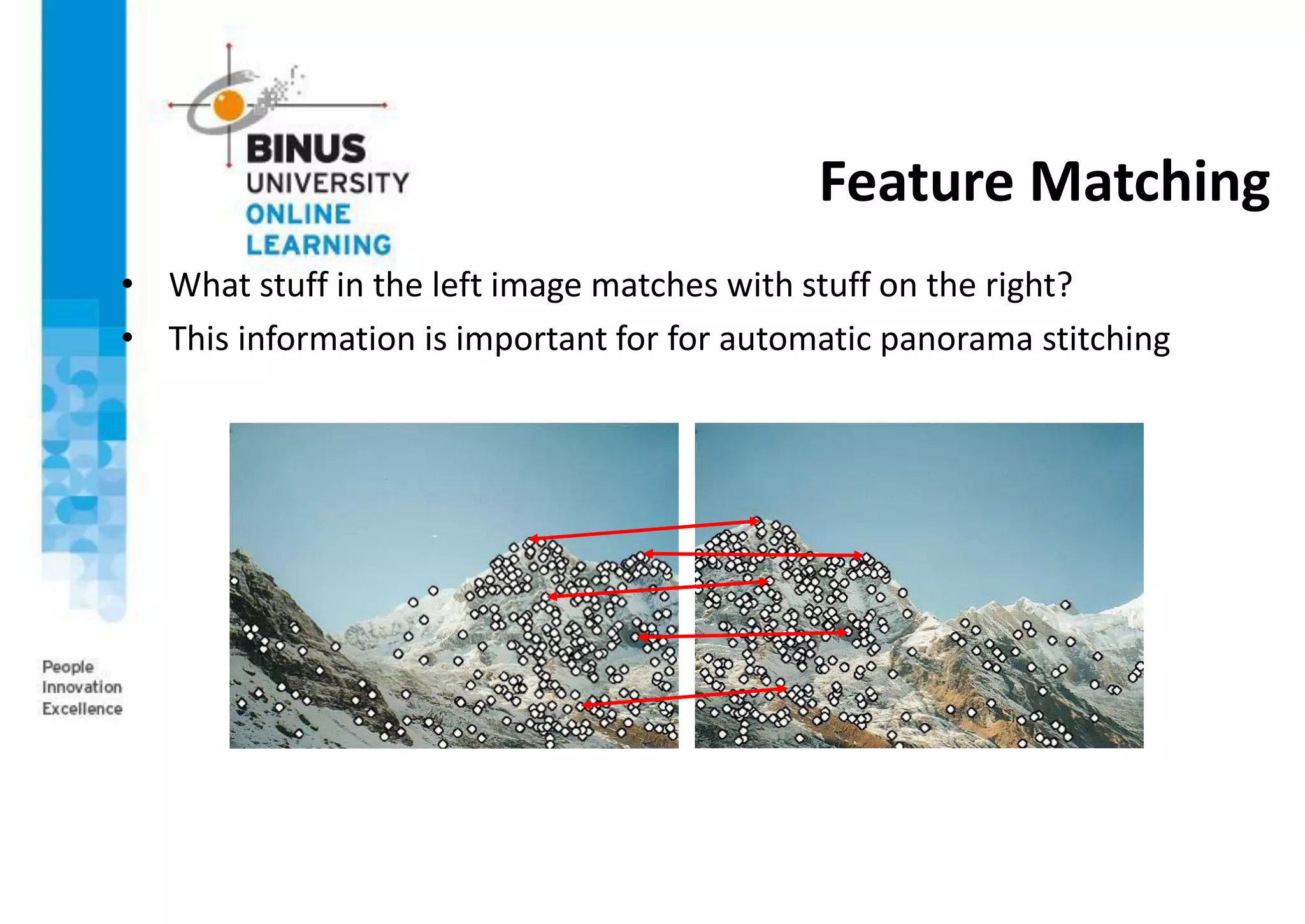
Feature Matching
• What stuff in the left image matches with stuff on the right?
• This information is important for for automatic panorama stitching
Harder Case
by Diva Sian by scgbt
Even Harder Case
NASA Mars Rover images with SIFT feature matches
Figure by Noah Snavely
Image Matching Procedure
1. Detection of distinguished regions
2. Local invariant description of these regions
3. Definition of the correspondence space
4. searching of a globally consistent subset of correspondences.
Invariant Features
Invariant Local Features
1. At an interesting
point, let’s define a
coordinate system
(x,y axis)
2. Use the coordinate
system to pull out a
patch at that point
Invariant Local Features
• Algorithm for finding points and representing their patches should produce similar
results even when conditions vary
• Buzzword is “invariance”
– Geometric invariance: translation, rotation, scale
– Photometric invariance: brightness, exposure, …etc.
Feature Descriptors
What makes good feature?
• We would like to align by matching local features of these 3 images
• What would be the good local features (ones easy to match)?
Local Measure of Uniqueness
Suppose we only consider a small window of pixels
• What defines whether a feature is a good or bad candidate?
• How does the window change when we shift it?
• Shifting the window in any direction causes a big change
“flat” region:
no change in all
directions
“edge”:
no change along
the edge direction
“corner”:
significant change
in all directions
Harris Corner Detector
(example)
Invariance
Suppose we are comparing two images I1 and I2
– I2 may be a transformed version of I1
– What kinds of transformations are we likely to encounter in
practice?
We’d like to find the same features regardless of the
transformation
– This is called transformational invariance
– Most feature methods are designed to be invariant to
• Translation, 2D rotation, scale
– They can usually also handle
• Limited 3D rotations (SIFT works up to about 60 degrees)
• Limited affine transformations (2D rotation, scale, shear)
• Limited illumination/contrast changes
How to achieve invariance?
1. Make sure our detector is invariant
– Harris is invariant to translation and rotation
– Scale is trickier
• common approach is to detect features at many scales using a Gaussian pyramid
(e.g., MOPS)
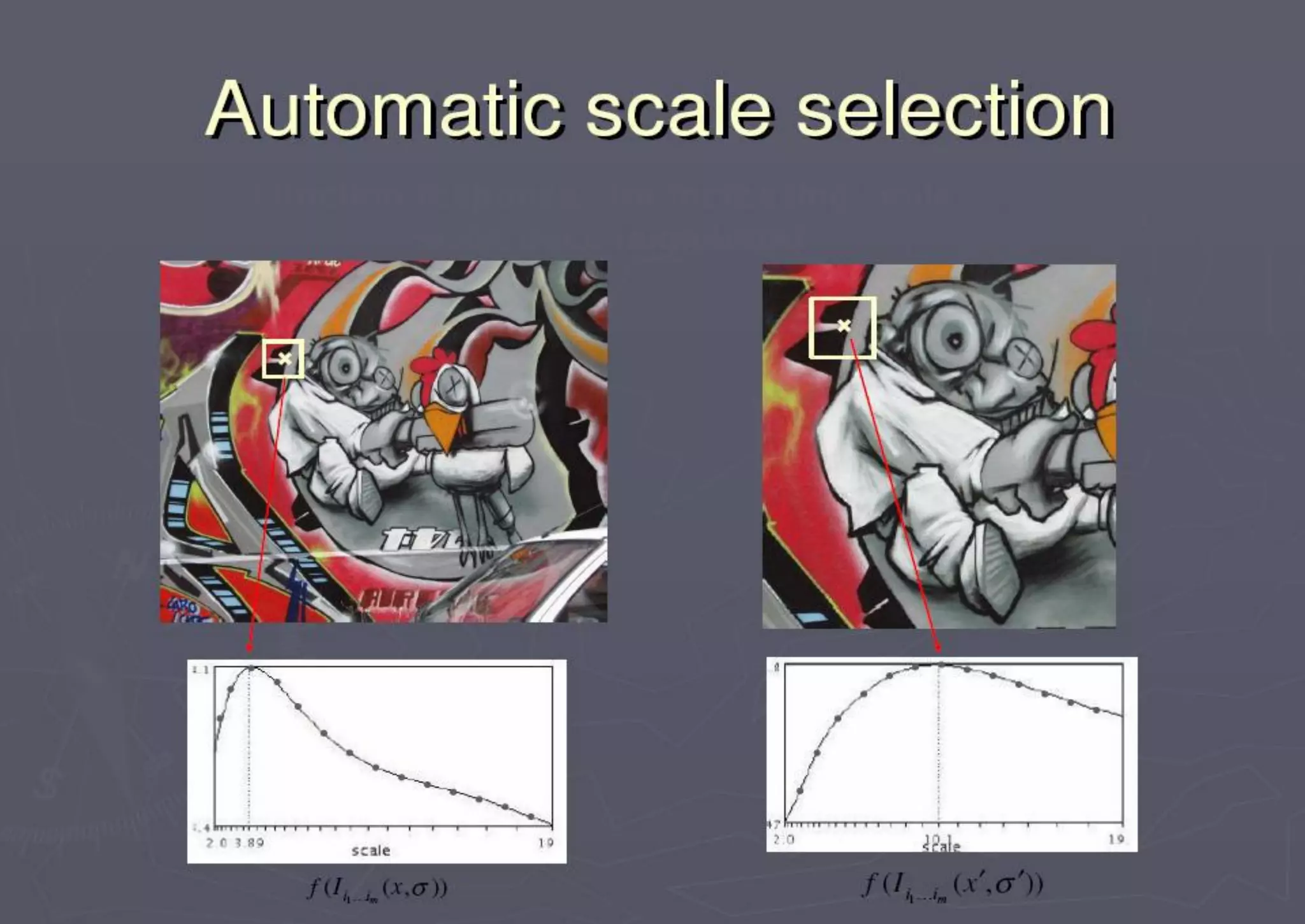
• More sophisticated methods find “the best scale” to represent each feature (e.g.,
SIFT)
2. Design an invariant feature descriptor
– A descriptor captures the information in a region around the
detected feature point
– The simplest descriptor: a square window of pixels
• What’s this invariant to?
– Let’s look at some better approaches…
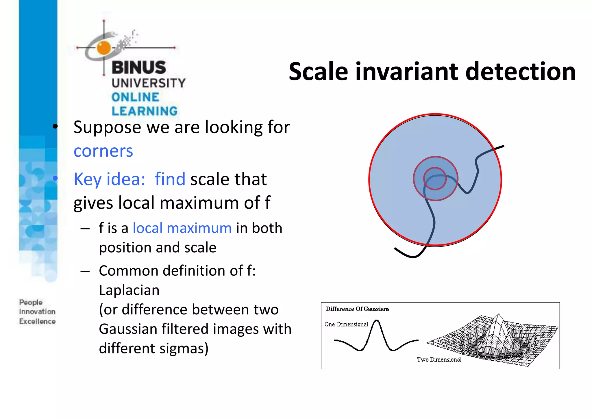
Scale invariant detection
• Suppose we are looking for
corners
• Key idea: find scale that
gives local maximum of f
– f is a local maximum in both
position and scale
– Common definition of f:
Laplacian
(or difference between two
Gaussian filtered images with
different sigmas)
Slide from Tinne Tuytelaars
Lindeberg et al, 1996
Slide from Tinne Tuytelaars
Lindeberg et al., 1996
Rotation invariance for feature
descriptors
Find dominant orientation of the image patch
• This is given by x+, the eigenvector of H corresponding to +
– + is the larger eigenvalue
• Rotate the patch according to this angle
Figure by Matthew Brown
Multiscale Oriented PatcheS
descriptor
Take 40x40 square window
around detected feature
• Scale to 1/5 size (using
prefiltering)
• Rotate to horizontal
• Sample 8x8 square
window centered at
feature
• Intensity normalize the
window by subtracting
the mean, dividing by the
standard deviation in the
window (both window I
and aI+b will match)
8 pixels
Detections at Multiple Scales
Scale Invariant Feature Transform
Scale Invariant Feature
Transform
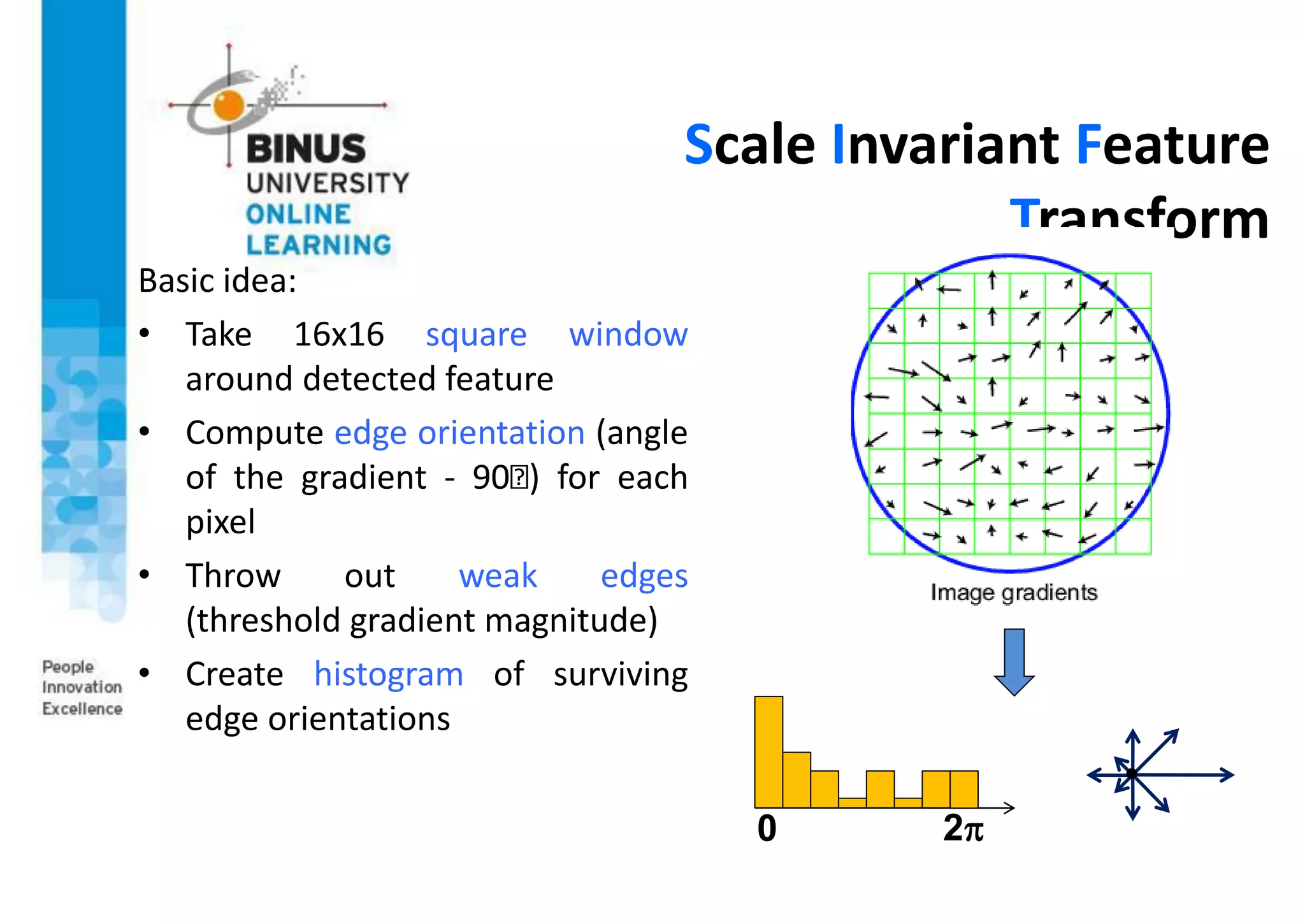
Basic idea:
• Take 16x16 square window
around detected feature
• Compute edge orientation (angle
of the gradient - 90 ) for each
pixel
• Throw out weak edges
(threshold gradient magnitude)
• Create histogram of surviving
edge orientations
0 2
SIFT Descriptor
Full version
• Divide the 16x16 window into a 4x4 grid of cells (2x2 case shown
below)
• Compute an orientation histogram for each cell
• 16 cells * 8 orientations = 128 dimensional descriptor
SIFT Properties
Extraordinarily robust matching technique
• Can handle changes in viewpoint
• Up to about 60 degree out of plane rotation
• Can handle significant changes in illumination, sometimes even day
vs. night (next example)
• Fast and efficient—can run in real time
• Lots of code available
http://people.csail.mit.edu/albert/ladypack/wiki/index.php?title=Kno
wn_implementations_of_SIFT
SIFT in Action
Feature Matching
Feature Matching
Given a feature in I1, how to find
the best match in I2?
1. Define distance function that
compares two descriptors
2. Test all the features in I2, find the one
with min distance
How to define the difference
between two features f1, f2?
• Simple approach is SSD(f1, f2)
– Sum of square differences between
entries of the two descriptors
– Can give good scores to very
ambiguous (bad) matches
I1
f1
f2
I2
Feature Distance
How to define the difference
between two features f1, f2?
• Better approach: ratio
distance = SSD(f1, f2) /
SSD(f1, f2’)
– f2 is best SSD match to f1 in I2
– f2’ is 2nd best SSD match to f1 in
I2
– gives small values for ambiguous
matches
f1
f2
f2’
I1
I2
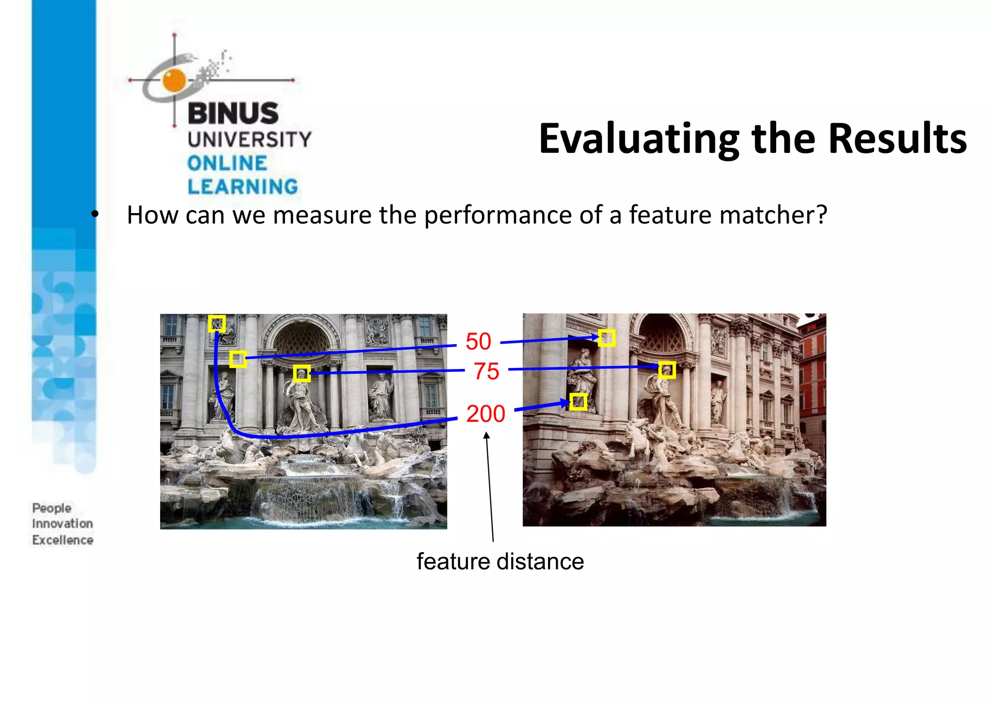
Evaluating the Results
• How can we measure the performance of a feature matcher?
50
75
200
feature distance
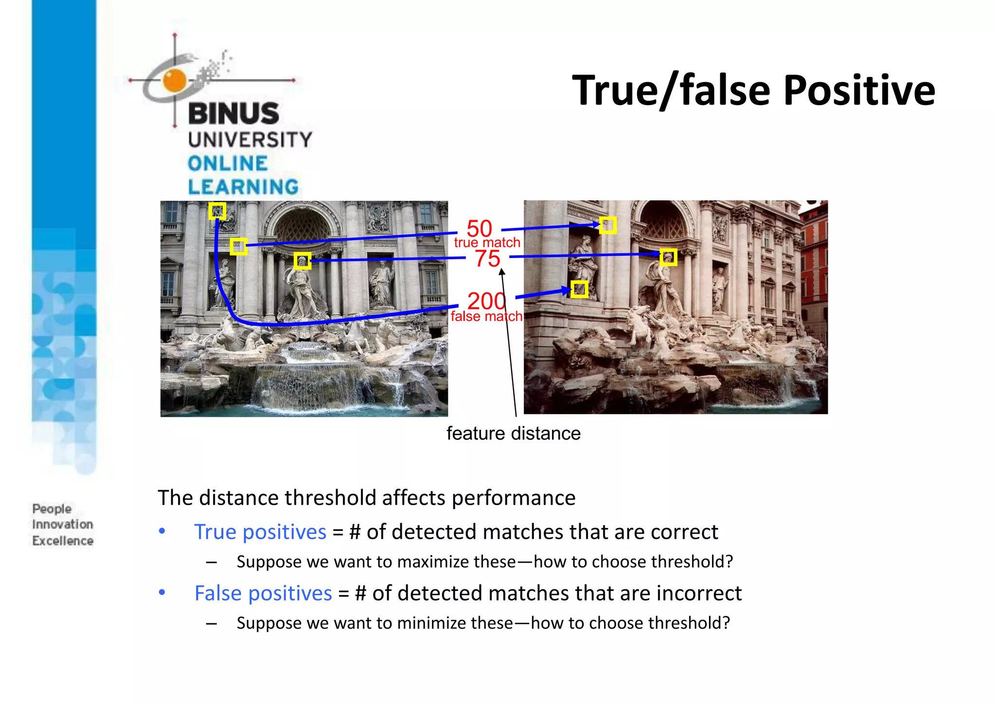
True/false Positive
The distance threshold affects performance
• True positives = # of detected matches that are correct
– Suppose we want to maximize these—how to choose threshold?
• False positives = # of detected matches that are incorrect
– Suppose we want to minimize these—how to choose threshold?
50
75
200
feature distance
false match
true match
Applications
Features are used for:
• Image alignment (e.g., mosaics)
• 3D reconstruction
• Motion tracking
• Object recognition
• Indexing and database retrieval
• Robot navigation
• … etc.
Acknowledgment
Some of slides in this PowerPoint presentation are adaptation from
various slides, many thanks to:
1. Deva Ramanan, Department of Computer Science, University of
California at Irvine (http://www.ics.uci.edu/~dramanan/)
Thank You

PPT s11-machine vision-s2

  • 1.
    Course: Machine Vision ImageMatching Session 12 D5627 – I Gede Putra Kusuma Negara, B.Eng., PhD
  • 2.
    Outline • Definition • Invariantfeatures • Scale Invariant Feature Transform • Feature matching
  • 3.
  • 4.
    Definition • Image matchingcan be defined as “the process of bringing two images geometrically into agreement so that corresponding pixels in the two images correspond to the same physical region of the scene being imaged • Image matching problem is accomplished by transforming (e.g., translating, rotating, scaling) one of the images in such a way that the similarity with the other image is maximized in some sense • The 3D nature of real-world scenarios makes this solution complex to achieve, specially because images can be taken from arbitrary viewpoints and in different illumination conditions.
  • 5.
    Image Matching • Imagematching is a fundamental aspect of many problems in computer vision, including object and scene recognition, content- based image retrieval, stereo correspondence, motion tracking, texture classification and video data mining. • It is a complex problem, that remains challenging due to partial occlusions, image deformations, and viewpoint or lighting changes that may occur across different images
  • 6.
    Image Matching (example) byDiva Sian by swashford
  • 7.
    Feature Matching • Whatstuff in the left image matches with stuff on the right? • This information is important for for automatic panorama stitching
  • 8.
    Harder Case by DivaSian by scgbt
  • 9.
    Even Harder Case NASAMars Rover images with SIFT feature matches Figure by Noah Snavely
  • 10.
    Image Matching Procedure 1.Detection of distinguished regions 2. Local invariant description of these regions 3. Definition of the correspondence space 4. searching of a globally consistent subset of correspondences.
  • 11.
  • 12.
    Invariant Local Features 1.At an interesting point, let’s define a coordinate system (x,y axis) 2. Use the coordinate system to pull out a patch at that point
  • 13.
    Invariant Local Features •Algorithm for finding points and representing their patches should produce similar results even when conditions vary • Buzzword is “invariance” – Geometric invariance: translation, rotation, scale – Photometric invariance: brightness, exposure, …etc. Feature Descriptors
  • 14.
    What makes goodfeature? • We would like to align by matching local features of these 3 images • What would be the good local features (ones easy to match)?
  • 15.
    Local Measure ofUniqueness Suppose we only consider a small window of pixels • What defines whether a feature is a good or bad candidate? • How does the window change when we shift it? • Shifting the window in any direction causes a big change “flat” region: no change in all directions “edge”: no change along the edge direction “corner”: significant change in all directions
  • 16.
  • 17.
    Invariance Suppose we arecomparing two images I1 and I2 – I2 may be a transformed version of I1 – What kinds of transformations are we likely to encounter in practice? We’d like to find the same features regardless of the transformation – This is called transformational invariance – Most feature methods are designed to be invariant to • Translation, 2D rotation, scale – They can usually also handle • Limited 3D rotations (SIFT works up to about 60 degrees) • Limited affine transformations (2D rotation, scale, shear) • Limited illumination/contrast changes
  • 18.
    How to achieveinvariance? 1. Make sure our detector is invariant – Harris is invariant to translation and rotation – Scale is trickier • common approach is to detect features at many scales using a Gaussian pyramid (e.g., MOPS) • More sophisticated methods find “the best scale” to represent each feature (e.g., SIFT) 2. Design an invariant feature descriptor – A descriptor captures the information in a region around the detected feature point – The simplest descriptor: a square window of pixels • What’s this invariant to? – Let’s look at some better approaches…
  • 19.
    Scale invariant detection •Suppose we are looking for corners • Key idea: find scale that gives local maximum of f – f is a local maximum in both position and scale – Common definition of f: Laplacian (or difference between two Gaussian filtered images with different sigmas)
  • 20.
    Slide from TinneTuytelaars Lindeberg et al, 1996 Slide from Tinne Tuytelaars Lindeberg et al., 1996
  • 22.
    Rotation invariance forfeature descriptors Find dominant orientation of the image patch • This is given by x+, the eigenvector of H corresponding to + – + is the larger eigenvalue • Rotate the patch according to this angle Figure by Matthew Brown
  • 23.
    Multiscale Oriented PatcheS descriptor Take40x40 square window around detected feature • Scale to 1/5 size (using prefiltering) • Rotate to horizontal • Sample 8x8 square window centered at feature • Intensity normalize the window by subtracting the mean, dividing by the standard deviation in the window (both window I and aI+b will match) 8 pixels
  • 24.
  • 25.
  • 26.
    Scale Invariant Feature Transform Basicidea: • Take 16x16 square window around detected feature • Compute edge orientation (angle of the gradient - 90 ) for each pixel • Throw out weak edges (threshold gradient magnitude) • Create histogram of surviving edge orientations 0 2
  • 27.
    SIFT Descriptor Full version •Divide the 16x16 window into a 4x4 grid of cells (2x2 case shown below) • Compute an orientation histogram for each cell • 16 cells * 8 orientations = 128 dimensional descriptor
  • 28.
    SIFT Properties Extraordinarily robustmatching technique • Can handle changes in viewpoint • Up to about 60 degree out of plane rotation • Can handle significant changes in illumination, sometimes even day vs. night (next example) • Fast and efficient—can run in real time • Lots of code available http://people.csail.mit.edu/albert/ladypack/wiki/index.php?title=Kno wn_implementations_of_SIFT
  • 29.
  • 30.
  • 31.
    Feature Matching Given afeature in I1, how to find the best match in I2? 1. Define distance function that compares two descriptors 2. Test all the features in I2, find the one with min distance How to define the difference between two features f1, f2? • Simple approach is SSD(f1, f2) – Sum of square differences between entries of the two descriptors – Can give good scores to very ambiguous (bad) matches I1 f1 f2 I2
  • 32.
    Feature Distance How todefine the difference between two features f1, f2? • Better approach: ratio distance = SSD(f1, f2) / SSD(f1, f2’) – f2 is best SSD match to f1 in I2 – f2’ is 2nd best SSD match to f1 in I2 – gives small values for ambiguous matches f1 f2 f2’ I1 I2
  • 33.
    Evaluating the Results •How can we measure the performance of a feature matcher? 50 75 200 feature distance
  • 34.
    True/false Positive The distancethreshold affects performance • True positives = # of detected matches that are correct – Suppose we want to maximize these—how to choose threshold? • False positives = # of detected matches that are incorrect – Suppose we want to minimize these—how to choose threshold? 50 75 200 feature distance false match true match
  • 35.
    Applications Features are usedfor: • Image alignment (e.g., mosaics) • 3D reconstruction • Motion tracking • Object recognition • Indexing and database retrieval • Robot navigation • … etc.
  • 36.
    Acknowledgment Some of slidesin this PowerPoint presentation are adaptation from various slides, many thanks to: 1. Deva Ramanan, Department of Computer Science, University of California at Irvine (http://www.ics.uci.edu/~dramanan/)
  • 37.