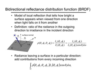
Review
• Pinhole projection model
• What are vanishing points and vanishing lines?
• What is orthographic projection?
• How can we approximate orthographic projection?
• Lenses
• Why do we need lenses?
• What is depth of field?
• What controls depth of field?
• What is field of view?
• What controls field of view?
• What are some kinds of lens aberrations?
• Digital cameras
• What are the two major types of sensor technologies?
• How can we capture color with a digital camera?
Assignment 1: Demosaicing
Historical context
• Pinhole model: Mozi (470-390 BCE),
Aristotle (384-322 BCE)
• Principles of optics (including lenses):
Alhacen (965-1039 CE)
• Camera obscura: Leonardo da Vinci
(1452-1519), Johann Zahn (1631-1707)
• First photo: Joseph Nicephore Niepce (1822)
• Daguerréotypes (1839)
• Photographic film: Eastman (1889)
• Cinema: Lumière Brothers (1895)
• Color Photography: Lumière Brothers (1908)
• Television: Baird, Farnsworth, Zworykin (1920s)
• First digitally scanned photograph: Russell Kirsch,
NIST (1957)
• First consumer camera with CCD:
Sony Mavica (1981)
• First fully digital camera: Kodak DCS100 (1990)
Niepce, “La Table Servie,” 1822
CCD chip
Alhacen’s notes
10 Early Firsts In Photography
http://listverse.com/history/top-10-incredible-
early-firsts-in-photography/
Early color photography
Sergey Prokudin-Gorsky (1863-1944)
Photographs of the Russian empire
(1909-1916)
http://www.loc.gov/exhibits/empire/
http://en.wikipedia.org/wiki/Sergei_Mikhailovich_Prokudin-Gorskii
Lantern
projector
“Fake miniatures”
Create your own fake miniatures: http://tiltshiftmaker.com/
http://tiltshiftmaker.com/tilt-shift-photo-gallery.php
Idea for class participation: if you find interesting (and
relevant) links, send them to me or (better yet) to the class
mailing list (comp776@cs.unc.edu).
Today: Capturing light
Source: A. Efros
Radiometry
What determines the brightness of an image
pixel?
Light source
properties
Surface
shape
Surface reflectance
properties
Optics
Sensor characteristics
Slide by L. Fei-Fei
Exposure
Solid Angle
• By analogy with angle (in radians), the solid angle
subtended by a region at a point is the area
projected on a unit sphere centered at that point
• The solid angle dω subtended by a patch of area dA
is given by:
2
cos
r
dA
d
θ
ω =
A
dA
Radiometry
• Radiance (L): energy carried by a ray
• Power per unit area perpendicular to the direction of travel,
per unit solid angle
• Units: Watts per square meter per steradian (W m-2 sr-1)
• Irradiance (E): energy arriving at a surface
• Incident power in a given direction per unit area
• Units: W m-2
• For a surface receiving radiance L(x,θ,φ) coming in from dω the
corresponding irradiance is
( ) ( ) ω
θ
φ
θ
φ
θ d
L
E cos
,
, =
n
θ
θ
cos
dA
dω
Radiometry of thin lenses
L: Radiance emitted from P toward P’
E: Irradiance falling on P’ from the lens
What is the relationship between E and L?
Forsyth & Ponce, Sec. 4.2.3
Example: Radiometry of thin lenses
α
cos
|
|
z
OP =
α
cos
'
|
'
|
z
OP =
4
2
d
π
δω
α
π
δ cos
4
2
⎟
⎟
⎠
⎞
⎜
⎜
⎝
⎛
=
d
L
P
L
z
d
z
d
L
E
⎥
⎥
⎦
⎤
⎢
⎢
⎣
⎡
⎟
⎠
⎞
⎜
⎝
⎛
=
⎟
⎟
⎠
⎞
⎜
⎜
⎝
⎛
= α
π
α
α
π
α 4
2
2
2
cos
'
4
)
cos
/
'
(
4
cos
cos
o
dA
dA’
Area of the lens:
The power δP received by the lens from P is
The irradiance received at P’ is
The radiance emitted from the lens towards dA’ is L
d
P
=
⎟
⎟
⎠
⎞
⎜
⎜
⎝
⎛
δω
α
π
δ
cos
4
2
Radiometry of thin lenses
• Image irradiance is linearly related to scene radiance
• Irradiance is proportional to the area of the lens and
inversely proportional to the squared distance between
the lens and the image plane
• The irradiance falls off as the angle between the
viewing ray and the optical axis increases
L
z
d
E
⎥
⎥
⎦
⎤
⎢
⎢
⎣
⎡
⎟
⎠
⎞
⎜
⎝
⎛
= α
π 4
2
cos
'
4
Forsyth & Ponce, Sec. 4.2.3
Radiometry of thin lenses
• Application:
• S. B. Kang and R. Weiss, Can we calibrate a camera using an
image of a flat, textureless Lambertian surface? ECCV 2000.
L
z
d
E
⎥
⎥
⎦
⎤
⎢
⎢
⎣
⎡
⎟
⎠
⎞
⎜
⎝
⎛
= α
π 4
2
cos
'
4
The journey of the light ray
• Camera response function: the mapping f from
irradiance to pixel values
• Useful if we want to estimate material properties
• Enables us to create high dynamic range images
Source: S. Seitz, P. Debevec
L
z
d
E
⎥
⎥
⎦
⎤
⎢
⎢
⎣
⎡
⎟
⎠
⎞
⎜
⎝
⎛
= α
π 4
2
cos
'
4
t
E
X Δ
⋅
=
( )
t
E
f
Z Δ
⋅
=
The journey of the light ray
• Camera response function: the mapping f from
irradiance to pixel values
Source: S. Seitz, P. Debevec
L
z
d
E
⎥
⎥
⎦
⎤
⎢
⎢
⎣
⎡
⎟
⎠
⎞
⎜
⎝
⎛
= α
π 4
2
cos
'
4
t
E
X Δ
⋅
=
( )
t
E
f
Z Δ
⋅
=
For more info
• P. E. Debevec and J. Malik. Recovering High Dynamic Range Radiance
Maps from Photographs. In SIGGRAPH 97, August 1997
The interaction of light and surfaces
What happens when a light ray hits a point on an object?
• Some of the light gets absorbed
– converted to other forms of energy (e.g., heat)
• Some gets transmitted through the object
– possibly bent, through “refraction”
• Some gets reflected
– possibly in multiple directions at once
• Really complicated things can happen
– fluorescence
Let’s consider the case of reflection in detail
• In the most general case, a single incoming ray could be reflected in
all directions. How can we describe the amount of light reflected in
each direction?
Slide by Steve Seitz
Bidirectional reflectance distribution function (BRDF)
• Model of local reflection that tells how bright a
surface appears when viewed from one direction
when light falls on it from another
• Definition: ratio of the radiance in the outgoing
direction to irradiance in the incident direction
• Radiance leaving a surface in a particular direction:
add contributions from every incoming direction
ω
θ
φ
θ
φ
θ
φ
θ
φ
θ
φ
θ
φ
θ
ρ
d
L
L
E
L
i
i
i
i
e
e
e
i
i
i
e
e
e
e
e
i
i
cos
)
,
(
)
,
(
)
,
(
)
,
(
)
,
,
,
( =
=
surface normal
( ) ( )
∫
Ω
i
i
i
i
i
e
e
i
i d
L ω
θ
φ
θ
φ
θ
φ
θ
ρ cos
,
,
,
,
,
BRDF’s can be incredibly complicated…
Diffuse reflection
• Light is reflected equally in all directions: BRDF is
constant
• Dull, matte surfaces like chalk or latex paint
• Microfacets scatter incoming light randomly
• Albedo: fraction of incident irradiance reflected by the
surface
• Radiosity: total power leaving the surface per unit area
(regardless of direction)
• Viewed brightness does not depend on viewing
direction, but it does depend on direction of
illumination
Diffuse reflection: Lambert’s law
( ) ( ) ( )
( )
x
S
x
N
x
x
B d
d ⋅
= ρ
)
(
N
S
B: radiosity
ρ: albedo
N: unit normal
S: source vector (magnitude
proportional to intensity of the source)
x
Specular reflection
• Radiation arriving along a source
direction leaves along the specular
direction (source direction reflected
about normal)
• Some fraction is absorbed, some
reflected
• On real surfaces, energy usually goes
into a lobe of directions
• Phong model: reflected energy falls of
with
• Lambertian + specular model: sum of
diffuse and specular term
( )
δθ
n
cos
Specular reflection
Moving the light source
Changing the exponent
Photometric stereo
Assume:
• A Lambertian object
• A local shading model (each point on a surface receives light
only from sources visible at that point)
• A set of known light source directions
• A set of pictures of an object, obtained in exactly the same
camera/object configuration but using different sources
• Orthographic projection
Goal: reconstruct object shape and albedo
Sn
???
S1
S2
Forsyth & Ponce, Sec. 5.4
Surface model: Monge patch
Forsyth & Ponce, Sec. 5.4
( ) ( )
( )
( ) ( )
( )
j
j
j
j
V
y
x
g
S
k
y
x
N
y
x
S
y
x
N
y
x
k
y
x
B
k
y
x
I
⋅
=
⋅
=
⋅
=
=
)
,
(
)
(
,
,
,
,
)
,
(
)
,
(
ρ
ρ
Image model
• Known: source vectors Sj and pixel values Ij(x,y)
• We also assume that the response function of
the camera is a linear scaling by a factor of k
• Combine the unknown normal N(x,y) and albedo
ρ(x,y) into one vector g, and the scaling constant
k and source vectors Sj into another vector Vj:
Forsyth & Ponce, Sec. 5.4
Least squares problem
• Obtain least-squares solution for g(x,y)
• Since N(x,y) is the unit normal, ρ(x,y) is given by the
magnitude of g(x,y) (and it should be less than 1)
• Finally, N(x,y) = g(x,y) / ρ(x,y)
)
,
(
)
,
(
)
,
(
)
,
(
2
1
2
1
y
x
g
V
V
V
y
x
I
y
x
I
y
x
I
T
n
T
T
n ⎥
⎥
⎥
⎥
⎥
⎦
⎤
⎢
⎢
⎢
⎢
⎢
⎣
⎡
=
⎥
⎥
⎥
⎥
⎦
⎤
⎢
⎢
⎢
⎢
⎣
⎡
M
M
(n × 1)
known known unknown
(n × 3) (3 × 1)
Forsyth & Ponce, Sec. 5.4
• For each pixel, we obtain a linear system:
Example
Recovered albedo Recovered normal field
Forsyth & Ponce, Sec. 5.4
Recall the surface is
written as
This means the normal
has the form:
Recovering a surface from normals
If we write the estimated
vector g as
Then we obtain values for
the partial derivatives of
the surface:
(x,y, f (x, y))
g(x,y) =
g1(x, y)
g2 (x, y)
g3(x, y)
⎛
⎝
⎜
⎜
⎞
⎠
⎟
⎟
fx (x,y) = g1(x, y) g3(x, y)
( )
fy(x, y) = g2(x,y) g3(x,y)
( )
N(x,y) =
1
fx
2
+ fy
2
+1
⎛
⎝
⎜
⎞
⎠
⎟
− fx
− fy
1
⎛
⎝
⎜
⎜
⎞
⎠
⎟
⎟
Forsyth & Ponce, Sec. 5.4
Recovering a surface from normals
Integrability: for the
surface f to exist, the
mixed second partial
derivatives must be equal:
We can now recover the
surface height at any point
by integration along some
path, e.g.
∂ g1(x, y) g3(x, y)
( )
∂y
=
∂ g2(x, y) g3(x, y)
( )
∂x
f (x, y) = fx (s, y)ds
0
x
∫ +
fy (x,t)dt
0
y
∫ + c
Forsyth & Ponce, Sec. 5.4
(for robustness, can take
integrals over many
different paths and
average the results)
(in practice, they should
at least be similar)
Surface recovered by integration
Forsyth & Ponce, Sec. 5.4
Limitations
• Orthographic camera model
• Simplistic reflectance and lighting model
• No shadows
• No interreflections
• No missing data
• Integration is tricky
Finding the direction of the light source
⎟
⎟
⎟
⎟
⎟
⎠
⎞
⎜
⎜
⎜
⎜
⎜
⎝
⎛
=
⎟
⎟
⎟
⎟
⎟
⎠
⎞
⎜
⎜
⎜
⎜
⎜
⎝
⎛
⎟
⎟
⎟
⎟
⎟
⎠
⎞
⎜
⎜
⎜
⎜
⎜
⎝
⎛
)
,
(
)
,
(
)
,
(
1
)
,
(
)
,
(
)
,
(
1
)
,
(
)
,
(
)
,
(
1
)
,
(
)
,
(
)
,
(
2
2
1
1
2
2
2
2
2
2
1
1
1
1
1
1
n
n
z
y
x
n
n
z
n
n
y
n
n
x
z
y
x
z
y
x
y
x
I
y
x
I
y
x
I
A
S
S
S
y
x
N
y
x
N
y
x
N
y
x
N
y
x
N
y
x
N
y
x
N
y
x
N
y
x
N
M
M
M
M
M
⎟
⎟
⎟
⎟
⎟
⎠
⎞
⎜
⎜
⎜
⎜
⎜
⎝
⎛
=
⎟
⎟
⎟
⎟
⎟
⎠
⎞
⎜
⎜
⎜
⎜
⎜
⎝
⎛
⎟
⎟
⎟
⎟
⎟
⎠
⎞
⎜
⎜
⎜
⎜
⎜
⎝
⎛
)
,
(
)
,
(
)
,
(
1
)
,
(
)
,
(
1
)
,
(
)
,
(
1
)
,
(
)
,
(
2
2
1
1
2
2
2
2
1
1
1
1
n
n
y
x
n
n
y
n
n
x
y
x
y
x
y
x
I
y
x
I
y
x
I
A
S
S
y
x
N
y
x
N
y
x
N
y
x
N
y
x
N
y
x
N
M
M
M
M
I(x,y) = N(x,y) ·S(x,y) + A
Full 3D case:
For points on the occluding contour:
P. Nillius and J.-O. Eklundh, “Automatic estimation of the projected light source
direction,” CVPR 2001
N
S
Finding the direction of the light source
P. Nillius and J.-O. Eklundh, “Automatic estimation of the projected light source
direction,” CVPR 2001
Application: Detecting composite photos
Fake photo
Real photo
Next time: Color
Phillip Otto Runge (1777-1810)

Lec03 light

  • 1.
    Review • Pinhole projectionmodel • What are vanishing points and vanishing lines? • What is orthographic projection? • How can we approximate orthographic projection? • Lenses • Why do we need lenses? • What is depth of field? • What controls depth of field? • What is field of view? • What controls field of view? • What are some kinds of lens aberrations? • Digital cameras • What are the two major types of sensor technologies? • How can we capture color with a digital camera?
  • 2.
  • 3.
    Historical context • Pinholemodel: Mozi (470-390 BCE), Aristotle (384-322 BCE) • Principles of optics (including lenses): Alhacen (965-1039 CE) • Camera obscura: Leonardo da Vinci (1452-1519), Johann Zahn (1631-1707) • First photo: Joseph Nicephore Niepce (1822) • Daguerréotypes (1839) • Photographic film: Eastman (1889) • Cinema: Lumière Brothers (1895) • Color Photography: Lumière Brothers (1908) • Television: Baird, Farnsworth, Zworykin (1920s) • First digitally scanned photograph: Russell Kirsch, NIST (1957) • First consumer camera with CCD: Sony Mavica (1981) • First fully digital camera: Kodak DCS100 (1990) Niepce, “La Table Servie,” 1822 CCD chip Alhacen’s notes
  • 4.
    10 Early FirstsIn Photography http://listverse.com/history/top-10-incredible- early-firsts-in-photography/
  • 5.
    Early color photography SergeyProkudin-Gorsky (1863-1944) Photographs of the Russian empire (1909-1916) http://www.loc.gov/exhibits/empire/ http://en.wikipedia.org/wiki/Sergei_Mikhailovich_Prokudin-Gorskii Lantern projector
  • 6.
    “Fake miniatures” Create yourown fake miniatures: http://tiltshiftmaker.com/ http://tiltshiftmaker.com/tilt-shift-photo-gallery.php Idea for class participation: if you find interesting (and relevant) links, send them to me or (better yet) to the class mailing list (comp776@cs.unc.edu).
  • 7.
  • 8.
    Radiometry What determines thebrightness of an image pixel? Light source properties Surface shape Surface reflectance properties Optics Sensor characteristics Slide by L. Fei-Fei Exposure
  • 9.
    Solid Angle • Byanalogy with angle (in radians), the solid angle subtended by a region at a point is the area projected on a unit sphere centered at that point • The solid angle dω subtended by a patch of area dA is given by: 2 cos r dA d θ ω = A
  • 10.
    dA Radiometry • Radiance (L):energy carried by a ray • Power per unit area perpendicular to the direction of travel, per unit solid angle • Units: Watts per square meter per steradian (W m-2 sr-1) • Irradiance (E): energy arriving at a surface • Incident power in a given direction per unit area • Units: W m-2 • For a surface receiving radiance L(x,θ,φ) coming in from dω the corresponding irradiance is ( ) ( ) ω θ φ θ φ θ d L E cos , , = n θ θ cos dA dω
  • 11.
    Radiometry of thinlenses L: Radiance emitted from P toward P’ E: Irradiance falling on P’ from the lens What is the relationship between E and L? Forsyth & Ponce, Sec. 4.2.3
  • 12.
    Example: Radiometry ofthin lenses α cos | | z OP = α cos ' | ' | z OP = 4 2 d π δω α π δ cos 4 2 ⎟ ⎟ ⎠ ⎞ ⎜ ⎜ ⎝ ⎛ = d L P L z d z d L E ⎥ ⎥ ⎦ ⎤ ⎢ ⎢ ⎣ ⎡ ⎟ ⎠ ⎞ ⎜ ⎝ ⎛ = ⎟ ⎟ ⎠ ⎞ ⎜ ⎜ ⎝ ⎛ = α π α α π α 4 2 2 2 cos ' 4 ) cos / ' ( 4 cos cos o dA dA’ Area of the lens: The power δP received by the lens from P is The irradiance received at P’ is The radiance emitted from the lens towards dA’ is L d P = ⎟ ⎟ ⎠ ⎞ ⎜ ⎜ ⎝ ⎛ δω α π δ cos 4 2
  • 13.
    Radiometry of thinlenses • Image irradiance is linearly related to scene radiance • Irradiance is proportional to the area of the lens and inversely proportional to the squared distance between the lens and the image plane • The irradiance falls off as the angle between the viewing ray and the optical axis increases L z d E ⎥ ⎥ ⎦ ⎤ ⎢ ⎢ ⎣ ⎡ ⎟ ⎠ ⎞ ⎜ ⎝ ⎛ = α π 4 2 cos ' 4 Forsyth & Ponce, Sec. 4.2.3
  • 14.
    Radiometry of thinlenses • Application: • S. B. Kang and R. Weiss, Can we calibrate a camera using an image of a flat, textureless Lambertian surface? ECCV 2000. L z d E ⎥ ⎥ ⎦ ⎤ ⎢ ⎢ ⎣ ⎡ ⎟ ⎠ ⎞ ⎜ ⎝ ⎛ = α π 4 2 cos ' 4
  • 15.
    The journey ofthe light ray • Camera response function: the mapping f from irradiance to pixel values • Useful if we want to estimate material properties • Enables us to create high dynamic range images Source: S. Seitz, P. Debevec L z d E ⎥ ⎥ ⎦ ⎤ ⎢ ⎢ ⎣ ⎡ ⎟ ⎠ ⎞ ⎜ ⎝ ⎛ = α π 4 2 cos ' 4 t E X Δ ⋅ = ( ) t E f Z Δ ⋅ =
  • 16.
    The journey ofthe light ray • Camera response function: the mapping f from irradiance to pixel values Source: S. Seitz, P. Debevec L z d E ⎥ ⎥ ⎦ ⎤ ⎢ ⎢ ⎣ ⎡ ⎟ ⎠ ⎞ ⎜ ⎝ ⎛ = α π 4 2 cos ' 4 t E X Δ ⋅ = ( ) t E f Z Δ ⋅ = For more info • P. E. Debevec and J. Malik. Recovering High Dynamic Range Radiance Maps from Photographs. In SIGGRAPH 97, August 1997
  • 17.
    The interaction oflight and surfaces What happens when a light ray hits a point on an object? • Some of the light gets absorbed – converted to other forms of energy (e.g., heat) • Some gets transmitted through the object – possibly bent, through “refraction” • Some gets reflected – possibly in multiple directions at once • Really complicated things can happen – fluorescence Let’s consider the case of reflection in detail • In the most general case, a single incoming ray could be reflected in all directions. How can we describe the amount of light reflected in each direction? Slide by Steve Seitz
  • 18.
    Bidirectional reflectance distributionfunction (BRDF) • Model of local reflection that tells how bright a surface appears when viewed from one direction when light falls on it from another • Definition: ratio of the radiance in the outgoing direction to irradiance in the incident direction • Radiance leaving a surface in a particular direction: add contributions from every incoming direction ω θ φ θ φ θ φ θ φ θ φ θ φ θ ρ d L L E L i i i i e e e i i i e e e e e i i cos ) , ( ) , ( ) , ( ) , ( ) , , , ( = = surface normal ( ) ( ) ∫ Ω i i i i i e e i i d L ω θ φ θ φ θ φ θ ρ cos , , , , ,
  • 19.
    BRDF’s can beincredibly complicated…
  • 20.
    Diffuse reflection • Lightis reflected equally in all directions: BRDF is constant • Dull, matte surfaces like chalk or latex paint • Microfacets scatter incoming light randomly • Albedo: fraction of incident irradiance reflected by the surface • Radiosity: total power leaving the surface per unit area (regardless of direction)
  • 21.
    • Viewed brightnessdoes not depend on viewing direction, but it does depend on direction of illumination Diffuse reflection: Lambert’s law ( ) ( ) ( ) ( ) x S x N x x B d d ⋅ = ρ ) ( N S B: radiosity ρ: albedo N: unit normal S: source vector (magnitude proportional to intensity of the source) x
  • 22.
    Specular reflection • Radiationarriving along a source direction leaves along the specular direction (source direction reflected about normal) • Some fraction is absorbed, some reflected • On real surfaces, energy usually goes into a lobe of directions • Phong model: reflected energy falls of with • Lambertian + specular model: sum of diffuse and specular term ( ) δθ n cos
  • 23.
    Specular reflection Moving thelight source Changing the exponent
  • 24.
    Photometric stereo Assume: • ALambertian object • A local shading model (each point on a surface receives light only from sources visible at that point) • A set of known light source directions • A set of pictures of an object, obtained in exactly the same camera/object configuration but using different sources • Orthographic projection Goal: reconstruct object shape and albedo Sn ??? S1 S2 Forsyth & Ponce, Sec. 5.4
  • 25.
    Surface model: Mongepatch Forsyth & Ponce, Sec. 5.4
  • 26.
    ( ) () ( ) ( ) ( ) ( ) j j j j V y x g S k y x N y x S y x N y x k y x B k y x I ⋅ = ⋅ = ⋅ = = ) , ( ) ( , , , , ) , ( ) , ( ρ ρ Image model • Known: source vectors Sj and pixel values Ij(x,y) • We also assume that the response function of the camera is a linear scaling by a factor of k • Combine the unknown normal N(x,y) and albedo ρ(x,y) into one vector g, and the scaling constant k and source vectors Sj into another vector Vj: Forsyth & Ponce, Sec. 5.4
  • 27.
    Least squares problem •Obtain least-squares solution for g(x,y) • Since N(x,y) is the unit normal, ρ(x,y) is given by the magnitude of g(x,y) (and it should be less than 1) • Finally, N(x,y) = g(x,y) / ρ(x,y) ) , ( ) , ( ) , ( ) , ( 2 1 2 1 y x g V V V y x I y x I y x I T n T T n ⎥ ⎥ ⎥ ⎥ ⎥ ⎦ ⎤ ⎢ ⎢ ⎢ ⎢ ⎢ ⎣ ⎡ = ⎥ ⎥ ⎥ ⎥ ⎦ ⎤ ⎢ ⎢ ⎢ ⎢ ⎣ ⎡ M M (n × 1) known known unknown (n × 3) (3 × 1) Forsyth & Ponce, Sec. 5.4 • For each pixel, we obtain a linear system:
  • 28.
    Example Recovered albedo Recoverednormal field Forsyth & Ponce, Sec. 5.4
  • 29.
    Recall the surfaceis written as This means the normal has the form: Recovering a surface from normals If we write the estimated vector g as Then we obtain values for the partial derivatives of the surface: (x,y, f (x, y)) g(x,y) = g1(x, y) g2 (x, y) g3(x, y) ⎛ ⎝ ⎜ ⎜ ⎞ ⎠ ⎟ ⎟ fx (x,y) = g1(x, y) g3(x, y) ( ) fy(x, y) = g2(x,y) g3(x,y) ( ) N(x,y) = 1 fx 2 + fy 2 +1 ⎛ ⎝ ⎜ ⎞ ⎠ ⎟ − fx − fy 1 ⎛ ⎝ ⎜ ⎜ ⎞ ⎠ ⎟ ⎟ Forsyth & Ponce, Sec. 5.4
  • 30.
    Recovering a surfacefrom normals Integrability: for the surface f to exist, the mixed second partial derivatives must be equal: We can now recover the surface height at any point by integration along some path, e.g. ∂ g1(x, y) g3(x, y) ( ) ∂y = ∂ g2(x, y) g3(x, y) ( ) ∂x f (x, y) = fx (s, y)ds 0 x ∫ + fy (x,t)dt 0 y ∫ + c Forsyth & Ponce, Sec. 5.4 (for robustness, can take integrals over many different paths and average the results) (in practice, they should at least be similar)
  • 31.
    Surface recovered byintegration Forsyth & Ponce, Sec. 5.4
  • 32.
    Limitations • Orthographic cameramodel • Simplistic reflectance and lighting model • No shadows • No interreflections • No missing data • Integration is tricky
  • 33.
    Finding the directionof the light source ⎟ ⎟ ⎟ ⎟ ⎟ ⎠ ⎞ ⎜ ⎜ ⎜ ⎜ ⎜ ⎝ ⎛ = ⎟ ⎟ ⎟ ⎟ ⎟ ⎠ ⎞ ⎜ ⎜ ⎜ ⎜ ⎜ ⎝ ⎛ ⎟ ⎟ ⎟ ⎟ ⎟ ⎠ ⎞ ⎜ ⎜ ⎜ ⎜ ⎜ ⎝ ⎛ ) , ( ) , ( ) , ( 1 ) , ( ) , ( ) , ( 1 ) , ( ) , ( ) , ( 1 ) , ( ) , ( ) , ( 2 2 1 1 2 2 2 2 2 2 1 1 1 1 1 1 n n z y x n n z n n y n n x z y x z y x y x I y x I y x I A S S S y x N y x N y x N y x N y x N y x N y x N y x N y x N M M M M M ⎟ ⎟ ⎟ ⎟ ⎟ ⎠ ⎞ ⎜ ⎜ ⎜ ⎜ ⎜ ⎝ ⎛ = ⎟ ⎟ ⎟ ⎟ ⎟ ⎠ ⎞ ⎜ ⎜ ⎜ ⎜ ⎜ ⎝ ⎛ ⎟ ⎟ ⎟ ⎟ ⎟ ⎠ ⎞ ⎜ ⎜ ⎜ ⎜ ⎜ ⎝ ⎛ ) , ( ) , ( ) , ( 1 ) , ( ) , ( 1 ) , ( ) , ( 1 ) , ( ) , ( 2 2 1 1 2 2 2 2 1 1 1 1 n n y x n n y n n x y x y x y x I y x I y x I A S S y x N y x N y x N y x N y x N y x N M M M M I(x,y) = N(x,y) ·S(x,y) + A Full 3D case: For points on the occluding contour: P. Nillius and J.-O. Eklundh, “Automatic estimation of the projected light source direction,” CVPR 2001 N S
  • 34.
    Finding the directionof the light source P. Nillius and J.-O. Eklundh, “Automatic estimation of the projected light source direction,” CVPR 2001
  • 35.
    Application: Detecting compositephotos Fake photo Real photo
  • 36.
    Next time: Color PhillipOtto Runge (1777-1810)