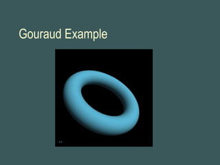
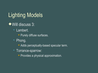
This document discusses lighting and shading techniques in computer graphics. It begins by distinguishing between lighting, which refers to light-matter interaction, and shading, which determines pixel colors. Three common lighting models are described: Lambert, Phong, and Torrance-Sparrow. For shading, it covers flat, Gouraud, and Phong shading. Gouraud shading improves on flat shading but can cause visual artifacts that Phong shading helps address by interpolating normals rather than colors at each pixel.

1. Lighting and Shading
Comp 770 Lecture Notes
Spring 2009

2. Overview
Last time, we covered light-matter interaction.
Now, apply it to rendering.
Outline:
 Lighting and shading.
 Lighting models.
 Shading methods.

3. Those Were the Days
(Or: how not to motivate a 21st
century computer
graphics paper.)
 “In trying to improve the quality of the synthetic images,
we do not expect to be able to display the object exactly
as it would appear in reality, with texture, overcast
shadows, etc. We hope only to display an image that
approximates the real object closely enough to provide a
certain degree of realism.”
– Bui Tuong Phong, 1975

4. Lighting vs. Shading
Commonly misused terms.
What’s the difference?

5. Lighting vs. Shading
Commonly misused terms.
What’s the difference?
Lighting designates the interaction between
materials and light sources, as in last lecture
( i.e. Physics).
Shading is the process of determining the color
of a pixel (i.e. Computer Graphics).
 Usually determined by lighting.
 Could use other methods: random color, NPR, etc.

6. Lighting Models
Will discuss 3:
 Lambert.
 Purely diffuse surfaces.
 Phong.
 Adds perceptually-based specular term.
 Torrance-sparrow:
 Provides a physical approximation.

7. Lambert Lighting Model
Sometimes mistakenly attributed to Gouraud.
 Gouraud didn’t introduce a new lighting model, just a
shading method.
 Used approximations from Warnock and Romney.
 Both based on Lambert’s cosine law.

8. Lambert’s Cosine Law
 The reflected luminous intensity in any direction from a
perfectly diffusing surface varies as the cosine of the
angle between the direction of incident light and the
normal vector of the surface.
 Intuitively: cross-sectional area of
the “beam” intersecting an element
of surface area is smaller for greater
angles with the normal.

9. Lambert’s Cosine Law
Ideally diffuse surfaces obey cosine law.
 Often called Lambertian surfaces.
Id = kdIincidentcos θ
= kdIincident(N·L).
 kd is the diffuse reflectance
of the material.
 Wavelength dependent, so usually specified as a color.
I
N
θ

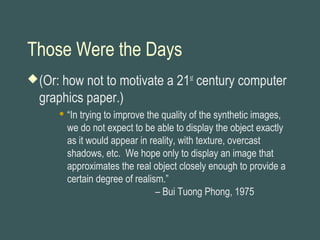
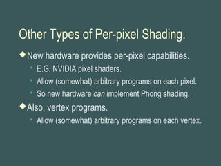
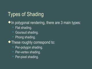
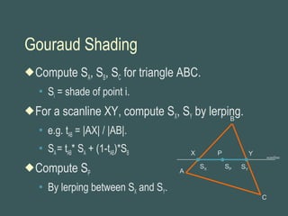
10. Phong Lighting Model
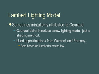
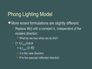
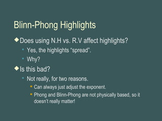
 Phong adds specular highlights.
 His original formula for the specular term:
 W(i)[cos s ]n
 s is the angle between the view and specular reflection directions.
 “W(i) is a function which gives the ratio of the specular reflected light
and the incident light as a function of the the incident angle i.”
• Ranges from 10 to 80 percent.
 “n is a power which models the specular reflected light for each
material.”
• Ranges from 1 to 10.

11. Phong Lighting Model
More recent formulations are slightly different.
 Replace W(i) with a constant ks, independent of the
incident direction.
 What do we lose when we do this?
 Is= ksIincidentcosn
φ
= ksIincident (V·R)n
.
 V is the view direction.
 R is the specular reflection direction.

12. Blinn-Phong Model
Popular variation of Phong model.
Uses the halfway vector, H.
Is = ksIincident (N·H)n
.
 H = L+V / | L+V |
What are the advantages?
L
N
φ φ
H
V

13. Blinn-Phong Model
Popular variation of Phong model.
Uses the halfway vector, H.
Is = ksIincident (N·H)n
.
 H = L+V / | L+V |
Faster to compute than reflection vector.
Still view-dependent since H depends on V.
L
N
φ φ
H
V

14. Blinn-Phong Highlights
Does using N.H vs. R.V affect highlights?
 Yes, the highlights “spread”.
 Why?
Is this bad?

15. Blinn-Phong Highlights
Does using N.H vs. R.V affect highlights?
 Yes, the highlights “spread”.
 Why?
Is this bad?
 Not really, for two reasons.
 Can always just adjust the exponent.
 Phong and Blinn-Phong are not physically based, so it
doesn’t really matter!

16. Torrance-Sparrow Model
 Introduced by Torrance and Sparrow in 1967 as a
theoretical model.
 Introduced to CG community by Blinn in 1977.
 same paper as “Halfway Vector” (Blinn-Phong).
 Attempts to provide a more physical model for specular
reflections from real surfaces.
 Points out that intensity of specular highlights is dependent
on the incident direction relative to normal.
 Phong attempted to model this with w(i) factor?

17. Torrance-Sparrow Model
Back to micro facets.
Assumptions:
 Diffuse component comes from multiple reflections
between facets and from internal scattering.
 Specular component of surface comes from facets
oriented in direction of H.

18. Torrance-Sparrow Model
Is= DGF / (N·V)
 D is the distribution function of the micro facet
directions on the surface.
 G is the amount that facets shadow and mask each
other.
 F is the Fresnel reflection law.

19. D: Micro Facet Distribution
T-S used simple Gaussian distribution:
 D = e -(ασ)
2
 α = deviation angle from halfway vector, H.
 σ = standard deviation.
 Large values = dull, small values = shiny

20. Denominator
Intensity proportional to number of facets in H
direction.
 So, must account for fact that observer sees more
surface area when surface is tilted.
 Change in area proportional to cosine of tilt angle.
 Hence, N·V in denominator.

21. G: Geometrical Attenuation Factor
Remember micro facet shadowing and masking?
Blinn derives this factor for symmetrical v-
shaped groove facets. (See paper).
shadow shadow
Masked Light

22. F: Fresnel Reflection
Fraction of light incident on a facet that is
actually reflected rather than absorbed.
Function of angle of incidence and index of
refraction.
 F(φ, η).
 For metals (large η), F(φ, η) nearly constant at 1.
 For non-metals (small η), F(φ, η) has exponential
appearance. Near zero for φ = 0, to 1 at φ = π / 2.

23. Shading
Have seen some methods for computing
lighting.
 Given normal, light direction, material properties.
 Non-diffuse models need view direction.
Now explore methods of applying that lighting
(or other color) to pixels of rasterized surface.

24. Types of Shading
In polygonal rendering, there are 3 main types:
 Flat shading.
 Gouraud shading.
 Phong shading.
These roughly correspond to:
 Per-polygon shading.
 Per-vertex shading.
 Per-pixel shading.

25. Flat Shading
Fast and simple.
Compute the color of a polygon.
Use that color on every pixel of the polygon.

26. Gouraud Shading
Still pretty fast and simple.
Gives better sense of form than flat shading for
many applications.
Basic Idea:
 Compute color at each vertex.
 Bi-linearly interpolate color for each interior pixel.

27. Gouraud Shading
Compute SA, SB, SC for triangle ABC.
 Si = shade of point i.
For a scanline XY, compute SX, SY by lerping.
 e.g. tAB = |AX| / |AB|.
 SA= tAB* SA + (1-tAB)*SB
Compute SP
 By lerping between SX and SY.
scanline
A
B
C
SX
X Y
SY
P
SP

28. Linear Interpolation Concerns
 Perspective projection complicates linear interpolation.
 Relationship between screen space distance and eye space
distance is nonlinear.
 Therefore, relationship between
interpolation in the two spaces is also
nonlinear.
 Thus, screen space linear interpolation
of colors (and texture coordinates)
results in incorrect values.
 Note: potential homework / test problem!

29. Perspectively-correct Interpolation
Could interpolate in eye space, then project
every interpolated point.
 Way too much work!
Can we interpolate in screen space and correct
for perspective nonlinearity?
 Yes!

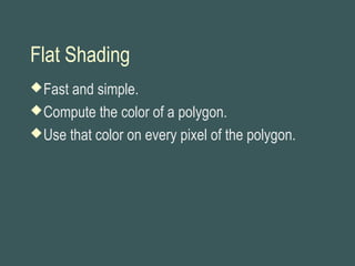
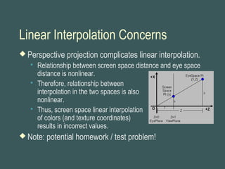
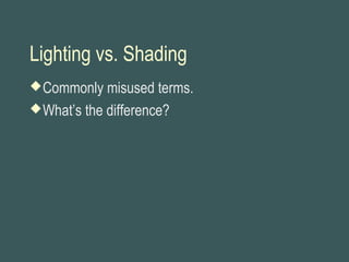
30. Perspectively-correct Interpolation
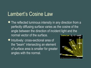
For a detailed derivation, see:
 http://www.cs.unc.edu/~hoff/techrep/persp/persp.html
Here, we skip to the punch line:
 Given two eye space points, E1 and E2.
 Can lerp in eye space: E(T) = E1(1-T) + E2(T).
 T is eye space parameter, t is screen space parameter.
 To see relationship, express in terms of screen
space t:
 E(t)= [ (E1/Z1)*(1-t) + (E2/Z2)*t ] / [ (1/Z1)*(1-t) + (1/Z2)*t ]

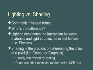
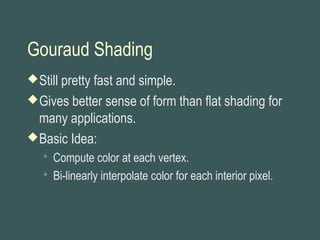
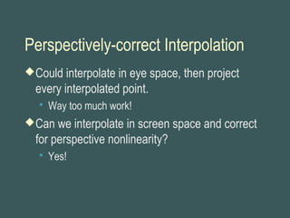
31. Perspectively-correct Interpolation
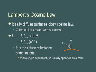
 E(t)= [ (E1/Z1)*(1-t) + (E2/Z2)*t ] / [ (1/Z1)*(1-t) + (1/Z2)*t ]
 E1/Z1, E2/Z2are projected points.
 Because Z1, Z2 are depths corresponding to E1, E2.
 Looking closely, can see that interpolation along an eye
space edge = interpolation along projected edge in
screen space divided by the interpolation of 1/Z.

32. Gouraud Example

33. Mach Bands
Gouraud discusses “artifact” of lerping.
Mach bands:
 Caused by interaction of neighboring retinal neurons.
 Acts as a sort of high-pass filter, accentuating
discontinuities in first derivative.
 Linear interpolation causes first deriv. Discontinuities
at polygon edges.

34. Mach Bands
Simple examples

35. Improvements
Gouraud suggests higher-order interpolation
would alleviate mach banding.
 But stresses the performance cost.
 Probably not worth it.
Phong shading helps the problem.

36. Phong Shading
Phong shading is not what earlier graphics
hardware implemented.
 APIs (D3D, OGL) employ Blinn-Phong lighting and
Gouraud shading.
Phong shading applies lighting computation per-
pixel.
 Uses linear interpolation of normal vectors, rather
than colors.

37. Phong Shading
Interpolation just as with colors in Gouraud
shading.
 Interpolate scan line endpoint normals Na, Nb from
endpoints of intercepted edges.
 Interpolate normal Np at each pixel from Na, Nb.
 Normalize Np.
 (Interpolation of unit vectors does not preserve length).
 Back-transform Npto eye space, compute lighting.

38. Phong Shading
Results are much improved over Gouraud.
 Harder to tell low- from high-polygon models.
 Still some indicators and problems:
 Silhouette still has a low tessellation.
 Shared vs. Unshared vertices.
 Mach banding.
• Yep, can still get first derivative discontinuities.

39. Other Types of Per-pixel Shading
Ray tracing.
 Doesn’t use Gouraud or Phong shading.
 Each pixel uses own ray to determine color.
 Can apply arbitrary lighting model.
 Classical (Whitted) ray tracing uses Phong model.
 Since ray tracing determines colors based on
intersections, don’t have to use polygonal geometry.
 Thus, can potentially use exact normals, rather than
interpolation.

40. Other Types of Per-pixel Shading.
New hardware provides per-pixel capabilities.
 E.G. NVIDIA pixel shaders.
 Allow (somewhat) arbitrary programs on each pixel.
 So new hardware can implement Phong shading.
Also, vertex programs.
 Allow (somewhat) arbitrary programs on each vertex.

41. References
Gouraud, Phong, Blinn papers I handed out.
 Available in Seminal Graphics, ACM press.
Glassner, Principles of Digital Image Synthesis,
volume two.
 Highly detailed and low level.
Möller and Haines, Real-Time Rendering.
 A great book, with the best bibliography you can find.

42. References
Rogers, Procedural Elements for Computer
Graphics.
 One of my favorites.
Foley, van dam, et al. Computer Graphics,
Principles and Practice.
 Not the best treatment, but it covers everything.