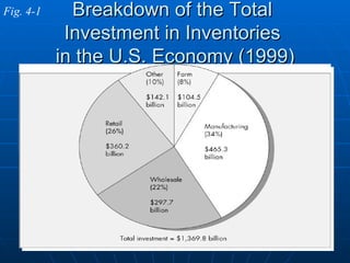
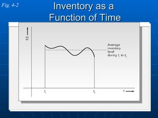
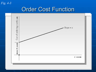
This document discusses inventory control for known demand. It introduces different types of inventories and reasons for holding inventory. It describes characteristics of inventory systems such as demand patterns and lead times. It outlines relevant inventory costs including holding, ordering, and penalty costs. It presents the economic order quantity (EOQ) model for determining optimal order quantities to minimize total inventory costs.

1. Chapter 4 Inventory Control Known Demand

2. Introduction Importance of inventory Types of inventories Motivation for holding inventories Characteristics of inventory systems Relevant costs

3. Importance of inventory Investment in inventories is enormous Companies that use scientific inventory control methods have a significant competitive advantage in the marketplace

4. Breakdown of the Total Investment in Inventories in the U.S. Economy (1999) Fig. 4-1

5. Types of inventories Raw materials Components WIP Finished goods Other (spare parts…)

6. Motivation for holding inventories Economies of scale ( setup cost ) Uncertainties: (demand, lead time, supply) Speculation (price increase) Transportation (pipeline inventories) Smoothing (seasonality) Logistics (supply, production, distribution) Control costs (large inv. Of inexpensive items)

7. Characteristics of inventory systems Demand Constant versus variable Known versus random Lead time Review time (continuous review, periodic review) Excess demand Backordered lost Changing inventory (perishability, obsolescence

8. Relevant costs Holding cost Warehousing (Providing space, Material handling, Labor) Taxes and insurance Spoilage, deterioration, and obsolescence Opportunity cost of alternative investment Ordering cost (setup cost)

9. Inventory as a Function of Time Fig. 4-2

10. Relevant costs (cont’d) Order cost Penalty cost (shortage cost)

11. Order Cost Function Fig. 4-3

12. Inventory Control The EOQ Model

13. Assumptions Demand rate λ (units per unit time) is known and constant Shortages are not permitted No lead time

14. Inventory Levels for the EOQ Model Fig. 4-4

15. Choose Q to minimize the average cost per unit time fixed+proportional order cost per cycle: K+cQ Cycle length: T=Q / λ Average inventory level per cycle: Q/2 Average cost per unit time: G(Q) = (K+cQ)/T + hQ/2 = K λ /Q+ λ c+hQ/2

16. The Average Annual Cost Function G(Q) Fig. 4-5

17. Reorder Point Calculation for Example 4.1 Fig. 4-6

18. Reorder Point Calculation for Lead Times Exceeding One Cycle Fig. 4-7

19. All-Units Discount Order Cost Function Fig. 4-9

20. Incremental Discount Order Cost Function Fig. 4-10

21. Average Annual Cost Function for Incremental Discount Schedule Fig. 4-12