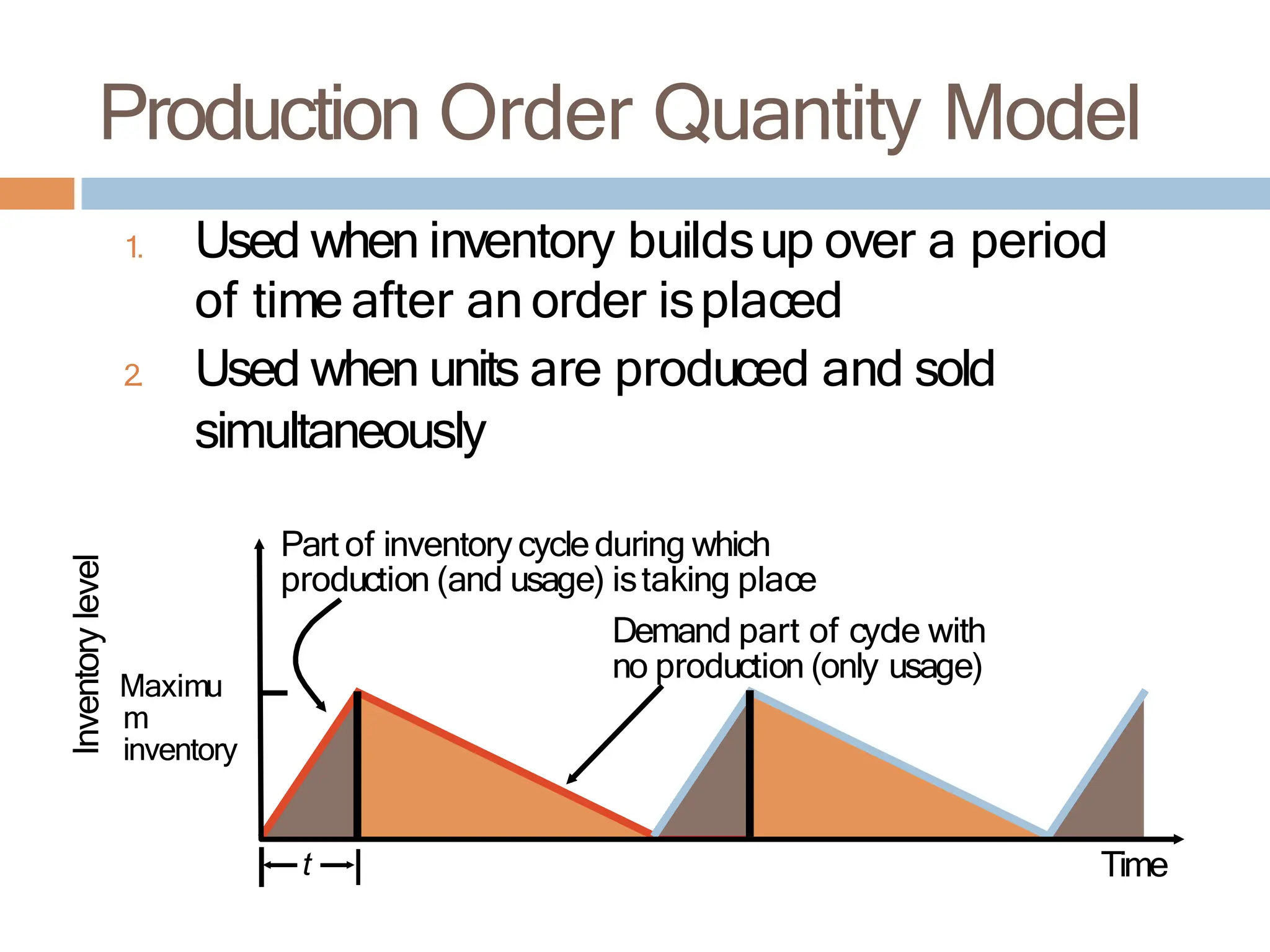
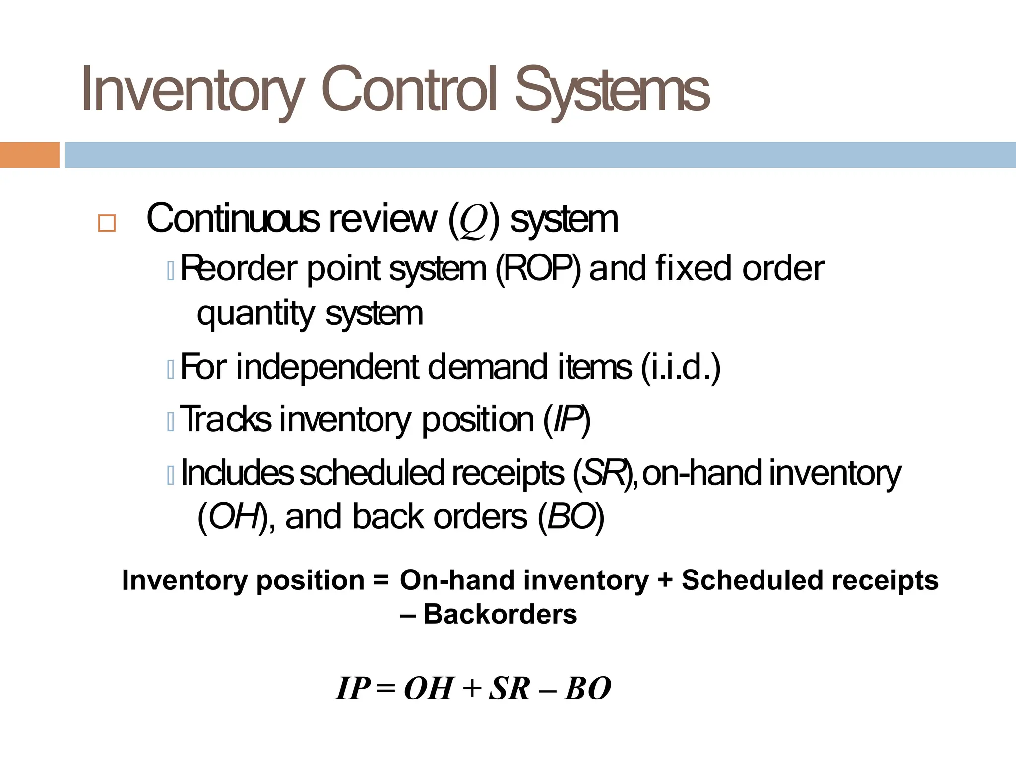
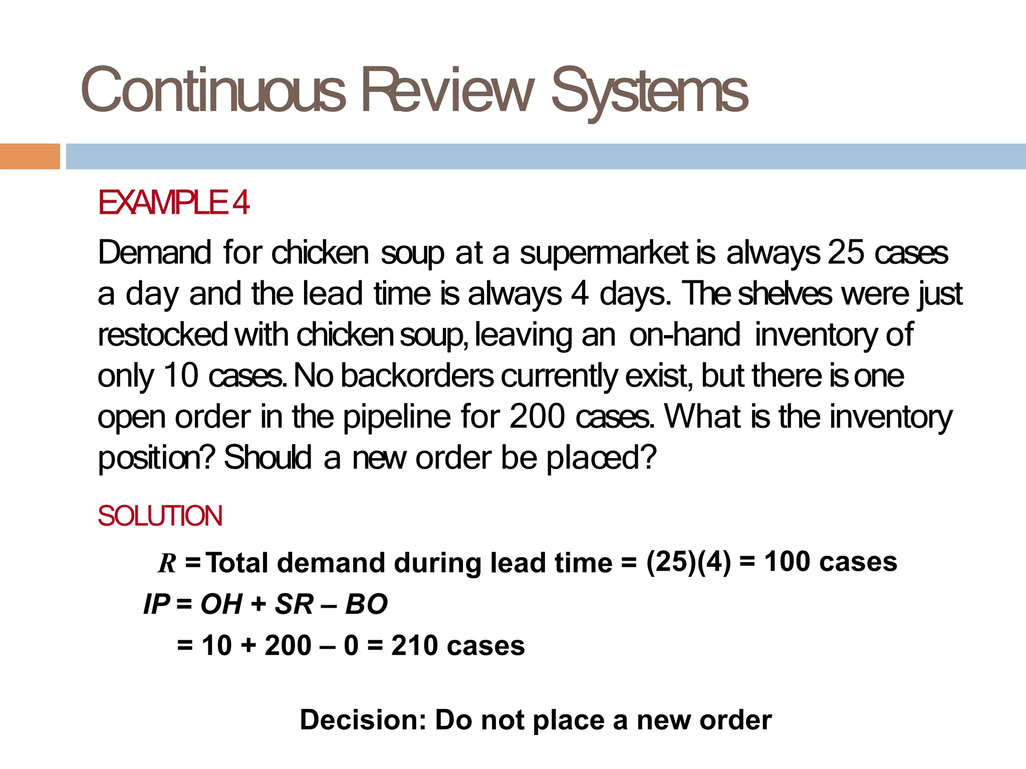
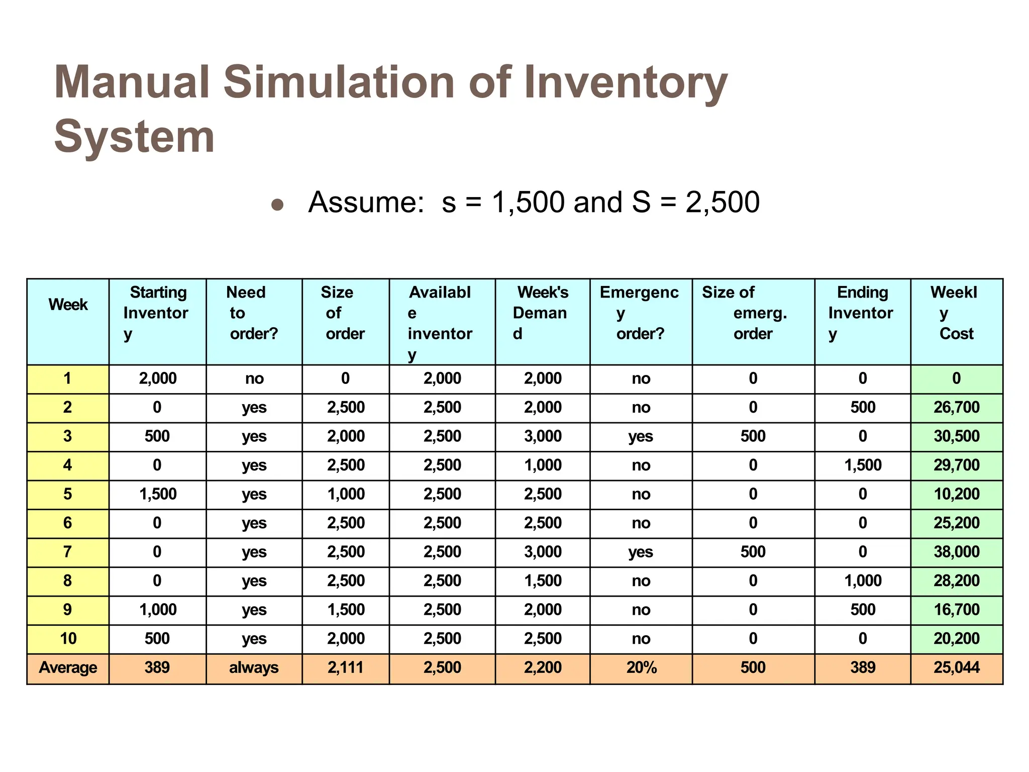
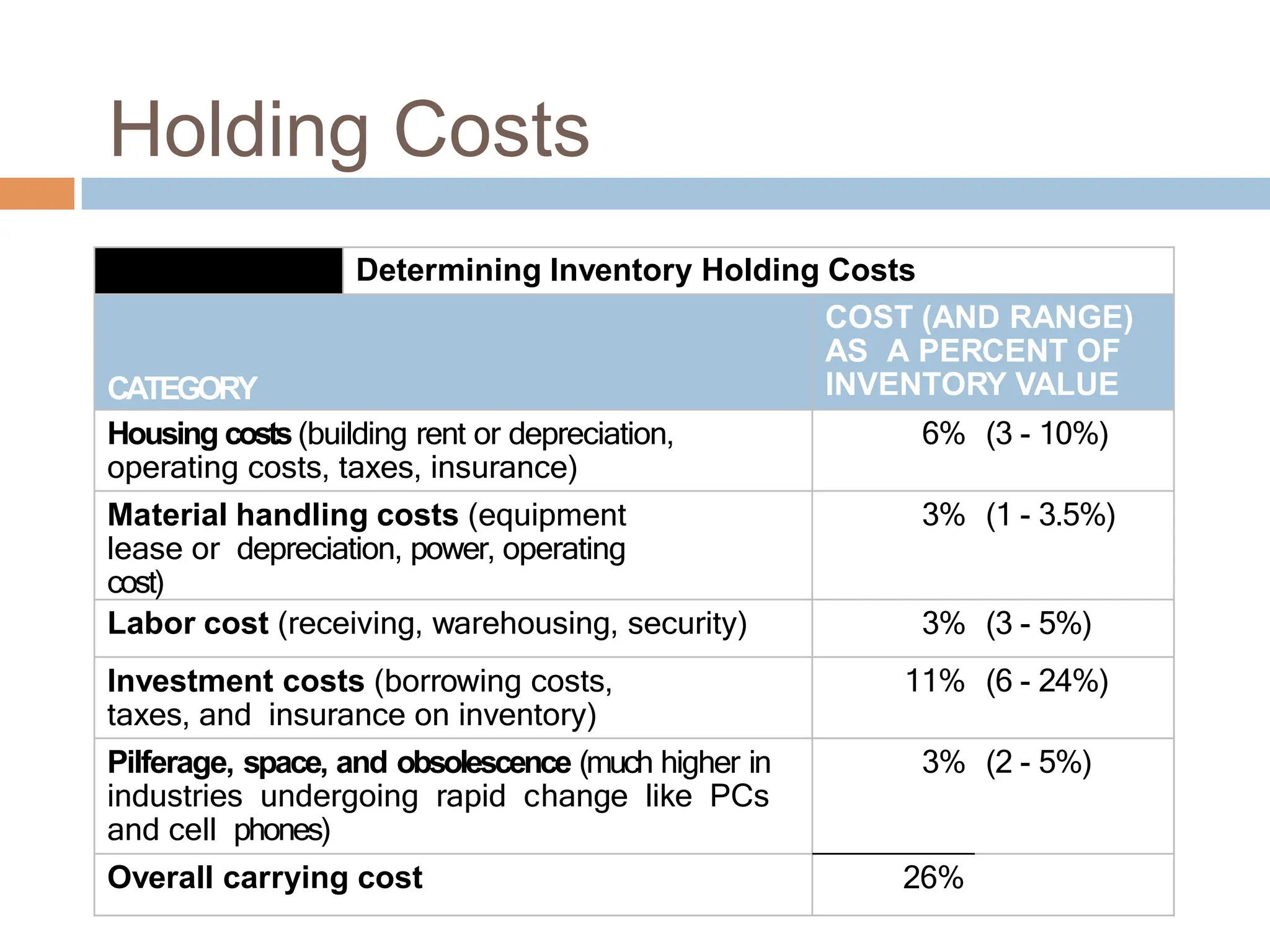
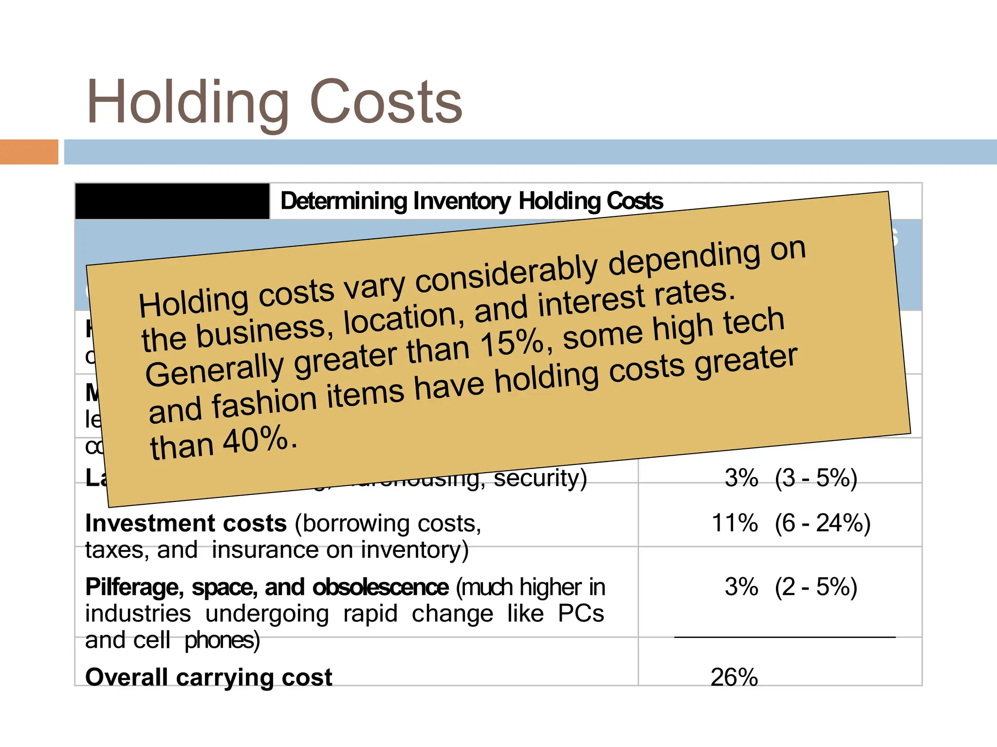
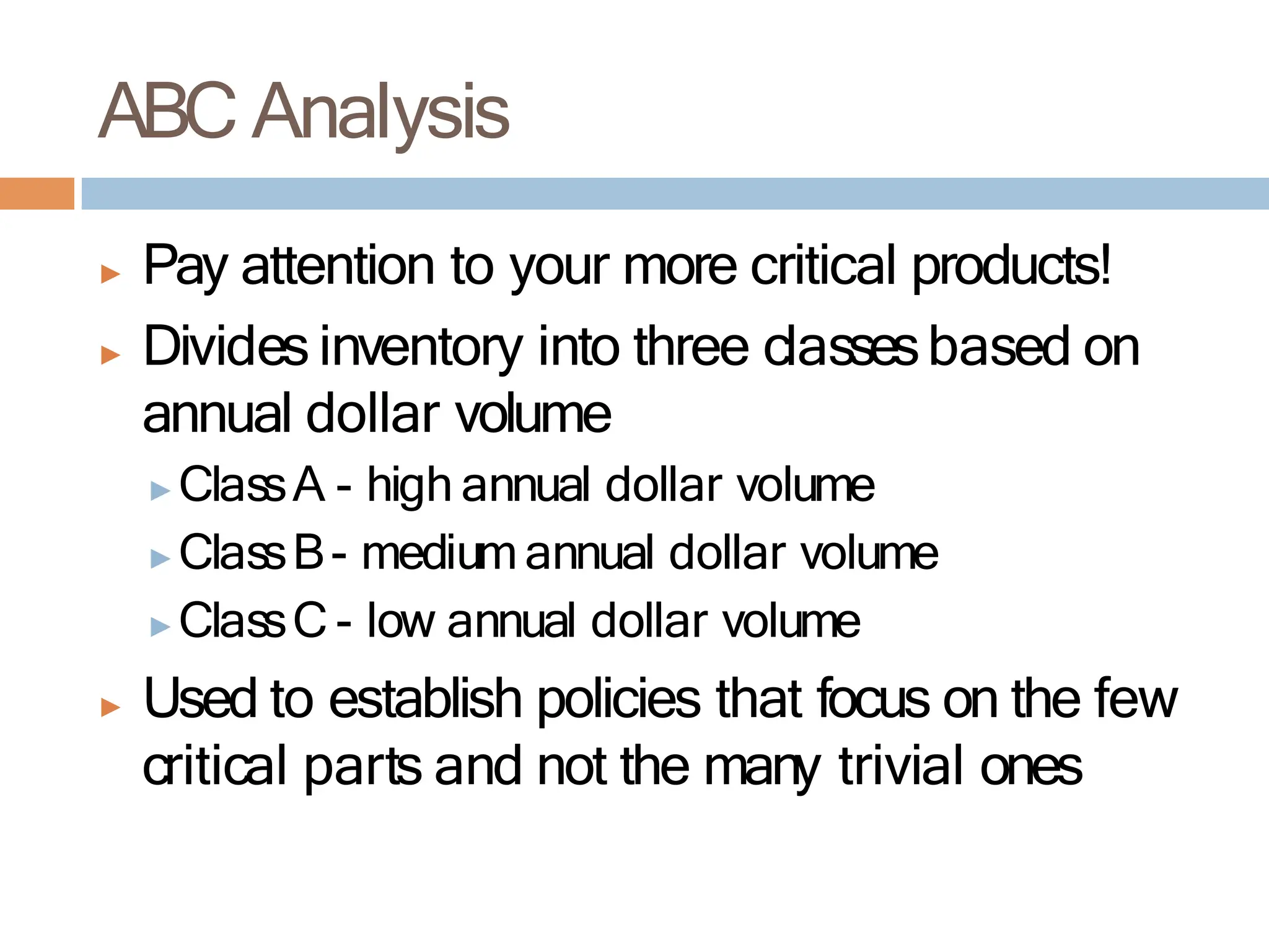
The document discusses inventory management, focusing on its importance, associated costs, and various inventory models including ABC analysis and Economic Order Quantity (EOQ). It highlights the significance of balancing inventory investments with customer service levels and examines factors impacting the decision to hold inventory. Additionally, it provides detailed methodologies for calculating optimal order quantities and total annual costs, enhancing the understanding of effective inventory control systems.

1. BIA 674 - Supply Chain Analytics
12.
Inventory Management

2. Outline
 The Importance of Inventory
 Inventory Costs
 ABC Analysis
 EOQ Models
 Probabilistic Models and Safety Stock
 Inventory Control Systems
 Single-Period Model
 Using Simulation for Inventory Management

3. What isInventory?
 Stock of items kept to meet future demand for
🞑 internal customers
🞑 external customers
 Purpose of inventory management
🞑 ORDERING POLICY: When and how many units to order
of each material when orders are placed with either
outsidesuppliersor production departments within
organizations?
🞑 ISSUINGPOLICY:howto issueunitsfrom inventory?
(FIFO, LIFO, random?)

4. Importance of Inventory
 Inventories are important to all types of firms:
🞑 They have to be counted, paid for, used in operations,
used to satisfy customers, and managed
🞑 T
oo much inventory reduces profitability
🞑 Too little inventory damages customer confidence
 It isoneof themostexpensiveassetsof many
companies representing asmuch as50% of total
invested capital
 It isone of the 3 most common reasons for
SME bankruptcy
 Need to balance inventory investment
and customer service

5. Why Do We Want to Hold Inventory
 Improve customer service
 Safe-guard to hazards in demand, supply, and delivery
that might cause stock-out
 T
ake advantage of economies of scale, & reduce:
🞑 ordering costs
🞑 Stock-out costs
🞑 acquisition costs
🞑 Fixed costs (e.g. fixed ordering costs)
 Contribute to the efficient and effective operation of
the production system, e.g.,
🞑 Reduces the number of costly set-ups and reschedulings
🞑 Smoothing and stabilizing resource utilization

6. Why We Do Not Want to Hold Inventory
 Certain costs increase such as
🞑 Storage costs
🞑 insurance costs
🞑 outdate costs
🞑 large-lot quality cost
🞑 cost of production problems
 Ties capital for which the company pays interest
 Hides productivity and quality problems
 Risk of getting stuck with unsalable goods

7. T
ypes of Inventory
▶ R
aw material
▶ Purchased but not processed
▶ Work-in-process (WIP)
▶ Undergone some change but not completed
▶ A function of cycle time for a product (e.g. items being
transported)
▶ Maintenance/repair/operating (MRO)
▶ Necessary to keep machinery and processes productive
▶ Finished goods
▶ Completed product awaiting shipment

8. The Material Flow Cycle
Input Wait for Wait to Move Wait in queue Setup Run Output
inspection be moved time for operator time time
Cycle time
95% 5%

9. Inventory and Service Quality
 Customers usually perceive quality service as
availability of goods they want when they want
them
 Inventory must be sufficient to provide high-quality
customer service

10. Inventory Costs

11. Inventory-Related Costs
 Ordering costs (unit variable costs & fixed ordering costs)
 costs of replenishing inventory, placing orders, receiving goods
 costs for to prepare a machine or process for manufacturing an order
 Holding or Inventory carrying costs
 cost of holding an item in inventory over time
 Shortage or Stock-out / penalty costs
🞑 How do you handle shortages?
🞑 Lost sales vs. backlogging
🞑 Watch out for service level
 Outdate costs (for perishable products)
 Opportunity costs

12. Holding Costs
Determining Inventory Holding Costs
CATEGORY
COST (AND RANGE)
AS A PERCENT OF
INVENTORY VALUE
Housing costs (building rent or depreciation,
operating costs, taxes, insurance)
6% (3 - 10%)
Material handling costs (equipment
lease or depreciation, power, operating
cost)
3% (1 - 3.5%)
Labor cost (receiving, warehousing, security) 3% (3 - 5%)
Investment costs (borrowing costs,
taxes, and insurance on inventory)
11% (6 - 24%)
Pilferage, space, and obsolescence (much higher in
industries undergoing rapid change like PCs
and cell phones)
3% (2 - 5%)
Overall carrying cost 26%

13. Holding Costs
Determining Inventory Holding Costs
CA
TEGOR
Y
COST(AND RANGE) AS
A PER
CENTOF
INVENTOR
Y VALUE
Housing costs(building rent or depreciation,
operating costs, taxes, insurance)
6% (3 - 10%)
Material handling costs (equipment
lease or depreciation, power, operating
cost)
3% (1 - 3.5%)
Labor cost (receiving, warehousing, security) 3% (3 - 5%)
Investment costs (borrowing costs,
taxes, and insurance on inventory)
11% (6 - 24%)
Pilferage, space, and obsolescence (much higher in
industries undergoing rapid change like PCs
and cell phones)
3% (2 - 5%)
Overall carrying cost 26%

14. ABC Analysis

15. ABC Analysis
▶ Pay attention to your more critical products!
▶ Divides inventory into three classesbased on
annual dollar volume
▶ClassA - high annual dollar volume
▶ClassB- mediumannual dollar volume
▶ClassC - low annual dollar volume
▶ Used to establish policies that focus on the few
critical parts and not the many trivial ones

16.  Concept: All items do not deserve the same
attention in termsof inventory management
 Focuson items that have the highest monetary value
 Step 1. Start with the inventoried items ranked by
dollar value in inventory in descending order
 Step2. Plot thecumulativedollar/euro valuein
inventory versus the cumulative items in inventory
ABC Analysis

17. ABC Analysis
10 20 30 40 50 60 70 80 90 100
Percentage of SKUs
Percentage
of
dollar
value
100 —
90 —
80 —
70 —
60 —
50 —
40 —
30 —
20 —
10 —
0 —
Class C
Class A
Class B
Typical Chart Using ABC Analysis
 ClassA
🞑 5 – 15 % of units
🞑 70 – 80 % of value
 ClassB
🞑 30 % of units
🞑 15 % of value
 ClassC
🞑 50 – 60 % of units
🞑 5 – 10 % of value

18. ABC AnalysisExample
ABC Calculation
(1) (2) (3) (4) (5) (6) (7)
PERCENT
OF PERCENT
ITEM NUMBER ANNUAL ANNUAL OF ANNUAL
STOCK OF ITEMS VOLUME UNIT DOLLAR DOLLAR
NUMBER STOCKED (UNITS) x COST = VOLUME VOLUME CLASS
#10286
#11526
20% 1,000
500
$ 90.00
154.00
$ 90,000
77,000
38.8%
33.2%
72%
A
A
#12760
#10867
#10500
30%
1,550
350
1,000
17.00
42.86
12.50
26,350
15,001
12,500
11.3%
6.4%
5.4%
23%
B
B
B
#12572 600 $ 14.17 $ 8,502 3.7% C
#14075 2,000 .60 1,200 .5% C
#01036 50% 100 8.50 850 .4% 5% C
#01307 1,200 .42 504 .2% C
#10572 250 .60 150 .1% C
8,550 $232,057 100.0%

19. B Items
| | | | | | | | | |
10 20 30 40 50 60 70 80 90 100
Percentage of inventory items
Percentage
of
annual
dollar
usage
80 –A Items
70 –
60 –
50 –
40 –
30 –
20 –
10 –
0 –
C Items
ABC Analysis

20. ▶ Other criteria than annual dollar volume may
be used
▶ High shortage or holding cost
▶ Anticipated engineering changes
▶ Delivery problems
▶ Quality problems
ABC Analysis

21. ▶ P
olicies employed may include
1. More emphasis on supplier development for A
items
2. Tighter physical inventory control for A items
3. More care in forecasting A items
ABC Analysis

22. EOQ Models

23. Ordering Policy under constant
demand
 Simple case
1. Demand rate is constant and known with certainty
2. Unit ordering cost = C
3. Every time an order is placed, there is a fixed cost = S
4. There isa unit holding cost = H
5. No constraints are placed on the size of each order
6
. The lead time iszero

24. t
 Company with steady rate of demand D = 100 tons/month
 Total annual demand = 1200 tons
 Purchase price C = $250/ton
 Delivery costs S= $50 (each time)
 Holding costs (storage, insurance, ...) H = $4/ton/month
Inventory
Level
• • •
Time
What iswrong with thismanagement?

25.  Irrational Ordering (time, quantity) ... why?
 Safety stock ... why?
Q
T 2T
t
Get rid of pre-conceived ideas …
3T

26. Inventory Usage Over Time
Order
quantity = Q
(maximum
inventory
level)
Usage rate
Average
inventory
on hand
QT
2
Minimum
inventory
Inventory
level
0
T
otal order received
2T
Time
T 3T

27. Objective is to minimize T
otal Annual Cost
Annual
cost
Order quantity
Total cost of
ordering + holding
inventory
Holding cost
Ordering (Setup)
cost
Minimum
total cost
Optimal order
quantity (Q*)
Determining the optimal cycle

28. Minimizing Costs
▶ By minimizing the sumof setup (or ordering)
and holding costs, total costs are minimized
▶ Optimal order size Q* will minimize total cost
▶ Optimal order quantity occurs when:
▶The derivative of the T
otal Cost with respect to the
order quantity isequal to zero
▶The holding cost and setup cost are equal

29. Calculating the Annual Costs
 Annual holding cost
Annual holding cost = (Average cycle inventory)
 (Unit holding cost)
 No of orders placed / year
 Annual ordering cost
Annual ordering cost = (Ordering cost / order)
 No of orders placed / year
 Total annual cycle-inventory cost
Total Annual costs = Annual holding cost
+ Annual ordering cost

30. Holding Cost / period
The cost of holding one unit in inventory for one cycle
= H (QT)/2
Ordering Cost / period
It isthe cost of ordering one lot with Q units
= CQ + S
Calculating all the costs
No. of orders / year
= Annual Demand / Oder Size = 12D/Q
T
otal Cost (C)
It isthe sumof annual holding and annual setup cost

31. Calculating the EOQ
 T
otal annual cycle-inventory cost
Where
TC = total annual cost
C = unit ordering annual cycle-inventory cost
Q = lot size
H = holding cost per unit per period
D = demand per period
S = fixed ordering or setup costs per lot
T = re-order period
TC = N (S + CQ) + H
QT
2
Fixed ordering
cost
Variable
ordering cost
Holding cost

32. Calculating the EOQ
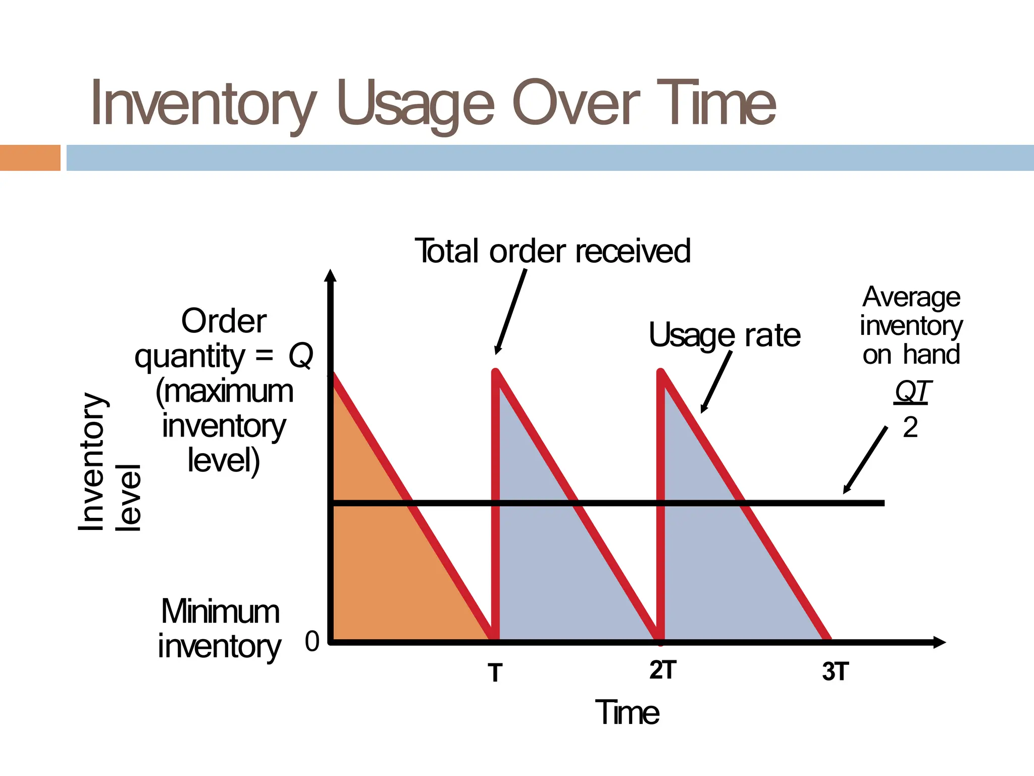
T
C = N[(S + CQ) + H(QT/2)]=
= (12DS/Q) + (12D/Q)CQ + (12D/Q)(HQ2/2D)=
=12DS/Q + 12DC + 6HQ
Tofind the optimal Quantity Q: Set derivative w.r.t Q = 0
Therefore,
-(12DS/Q2)+6H = 0 The optimal - order- quantity
Q* = 2SD/H = 50 tons
T = 0,5 month

33. Determine the optimal number of units to order
D = 1,000 units per year
S = $10 per order
H = $.50 per unit per year
Q*

2DS
H
Q*

0.50
2(1,000)(10)
 40,000  200 units
An EOQ Example

34. Determine expected number of orders
Q* = 200 units
D = 1,000 units
S = $10 per order
H = $.50 per unit per year
N = = 5 orders per year
1,000
200
= N =
Expected
number of
orders
Demand
Order quantity
D
=
Q*
An EOQ Example

35. An EOQ Example
Determine optimal time between orders
Q* = 200 units
N = 5 orders/year
D = 1,000 units
S = $10 per order
H = $.50 per unit per year
T = = 50 days between orders
250
5
= T =
Expected time
between
orders
Number of working days per year
Expected number of orders

36. Determine the total annual cost
D = 1,000 units
S= $10 per order
H = $.50 per unit per year
Q* = 200 units
N = 5 orders/year
T = 50 days
T
otal annual cost = Setup cost + Holding cost
TC  D S  Q H
Q 2
1,000

200
($10)
200
2
($.50)
 (5)($10)(100)($.50)
 $50$50  $100
Note: the cost of materials is not included, as it is assumed that the demand will
be satisfied and therefore it isa fixed cost
An EOQ Example

37. Calculating EOQ
EXAMPLE1
Amuseumof natural history opened a gift shopwhichoperates
52 weeks per year. Managing inventories hasbecome a
problem. Top-selling SKUisa bird feeder. Salesare 18 units
per week, the supplier charges $60 per unit. Ordering cost
is $45. Annual holding cost is 25 percent of a feeder’s value.
Management chose a 390-unit lot size.
What is the annual cycle-inventory cost of the current policy of
using a 390-unit lot size?
Would a lot size of 468 be better?

38. Calculating EOQ
SOLUTION
We begin by computing the annual demand and holding cost as
D = (18 units/week)(52 weeks/year) = 936 units
H = 0.25($60/unit) = $15
The total annual cycle-inventory cost for the current policy is
2 Q
Q D 390 936
C = (H) + (S) = ($15) + ($45)
2 390
= $2,925 + $108 = $3,033
The total annual cycle-inventory cost for the alternative lot size is
C =
468
($15) +
936
($45) = $3,510 + $90 = $3,600
2 468

39. Calculating the EOQ
3000 –
2000 –
1000 –
0 – | | |
Annual
cost
(dollars)
Current
cost
Lowest
cost
| | | | |
50 100 150 200 250 300 350 400
Best Q Lot Size (Q) Current
(EOQ) Q
cost
Total
=
Q
(H) + D (S)
2 Q
Total Annual Cycle-Inventory Cost Function for
the Bird Feeder
Ordering cost = D (S)
Q
Q
Holding cost = 2 (H)

40. Finding the EOQ, T
otal Cost, TBO
EXAMPLE2
Forthebird feeders inExample 1, calculate theEOQand its
total annual cycle-inventory cost. How frequently will orders be
placed if the EOQ isused?
SOLUTION
Using the formulasfor EOQ and annual cost, we get
EOQ = =
2DS
H
= 74.94 or 75 units
2(936)(45)
15

41. Finding the EOQ, T
otal Cost, TBO
Thetotal annual costismuchlessthan the$3,033 costof the
current policy of placing 390-unit orders.

42. Finding the EOQ, T
otal Cost, TBO
When the EOQ is used, the TBO can be expressed in various
ways for the same time period.
EOQ
EOQ
TBO = D =
75
= 0.080 year
936
EOQ D
EOQ 75
TBO = (12 months/year) = (12) = 0.96 month
EOQ D
EOQ 75
TBO = (52 weeks/year) = (52) = 4.17 weeks
EOQ D
EOQ 75
TBO = (365 days/year) = (365) = 29.25 days
936
936
936

43. Finding the EOQ, T
otal Cost, TBO
EXAMPLE3
Suppose that you are reviewing the inventory policies on an $80
item stocked at a hardware store. The current policy is to replenish
inventory by ordering in lots of 360 units. Additional information is:
D = 60 units per week, or 3,120 units per year
S = $30 per order
H = 25% of selling price, or $20 per unit per year
What isthe
EOQ? SOLUTION
EOQ = =
2DS
H
2(3,120)(30) = 97 units
20

44. Finding the EOQ, T
otal Cost, TBO
What is the total annual cost of the current policy (Q = 360),
and how does it compare with the cost with using the EOQ?
Current Policy EOQ Policy
Q = 360 units Q = 97 units
C = (360/2)(20) + (3,120/360)(30) C = (97/2)(20) + (3,120/97)(30)
C = 3,600 + 260 C = 970 + 965
C = $3,860 C = $1,935

45. Finding the EOQ, T
otal Cost, TBO
What isthe time between orders (TBO) for the current policy
and the EOQ policy, expressed in weeks?
360
TBO = 360 (52 weeks per year) = 6 weeks
EOQ
TBO = 97 (52 weeks per year) = 1.6 weeks
3,120
3,120

46. Managerial Insights
SENSITIVITY ANALYSIS OF THE EOQ
Parameter EOQ Parameter
Change
EOQ
Change
Comments
Demand 2DS
H
↑
↓
↓
↑
↓
↑
Increase in lot size is in proportion
to the square root of D.
Order/Setup
Costs
2DS
H
Weeks of supply decreases and
inventory turnover increases because
the lot size decreases.
Holding
Costs
2DS
H
Larger lots are justified when holding
costs decrease.

47. Robustness
▶ The EOQ model isrobust
▶ It works even if all parameters and
assumptionsare not met
▶ The total cost curve isrelatively flat in the
area of the EOQ

48. Introducing delivery lag
 EOQ answers the “how much” question
 The reorder point (ROP) tells“when” to order
 Lead time (L) isthe time between placing
and receiving an order
ROP =
Lead time for a new
order in days
Demand
per day
= d x L
d = D
Number of working days in a year

49. R
eorder P
oint Curve
Q*
ROP
(units)
Inventory
level
(units)
Time (days)
Lead time = L
Resupply takes place as order arrives
Slope = units/day = d

50. R
eorder P
oint Example
Demand = 8,000 iPods per year
250 working day year
Lead time for orders is 3 working days, but it may also
take 4 days
d =
D
Number of working days in a year
= 8,000/250 = 32 units
ROP = d x L
= 32 units per day x 3 days = 96 units
= 32 units per day x 4 days = 128 units

51. Introducing volume discounts
 Acompanybuysre-writable DVDs(10 disks/ box)
from a large mail-order distributor
 Thecompanyusesapproximately 5,000 boxes/ year
at a fairly constant rate
 The distributor offers the following quantity
discount schedule:
🞑 If <500 boxes are ordered, then cost = $10/box
🞑 If >500 but <800 boxes are ordered, then cost = $9.50
🞑 If >800 boxes are ordered, then cost = $9.25
 Fixed cost of purchasing = $25, and the cost of
capital = 12% per year. There is no storage cost.

52.  Solve 3 EOQ models
 Each one will hold for the corresponding region; if it does not
correspond, choose the lowest one that does
 Select the one with the lowest cost
Stepsin analyzing a quantity discount
1. For each discount, calculate Q*
2. If Q* for a discount doesn’t qualify, choose the lowest possible
quantity to get the discount
3. Compute the total cost for each Q* or adjusted value from
Step 2
4. Select the Q* that gives the lowest total cost
Introducing volume discounts

53. Quantity Discount Models
500 800
Order quantity
Total
cost
$
0
Q* for discount 2 is below the allowable range at point a and
must be adjusted upward to 500 units at point b
a
b
1st price
break
2nd price
break
Total cost
curve for
discount 1
Total cost curve for discount 2
Total cost curve for discount 3

54.  A company is a mail-order distributor of audio CDs
 They sell about 50,000 CDs/ year
 Each CD ispackaged in a jewel box they buy from a supplier
 Fixed cost for an order of boxes = $100; variable cost = $0.50,
storage cost = $0.50/unit/year, and cost of money is 10%
 Thecompanyassumesthat shortages are allowed, and lost demand
is backlogged … it just gets to the customer a little later (!)
 The company assigns a “penalty” of $1 for every week that a box
is delivered late, so annual shortage cost (penalty) p = $52/unit.
Allowing shortages

55. Allowing shortages
Q/D
b
(Q-b)/D b/D
 Allow shortages up to b units
 Order quantity Q
 Order-up-to inventory = Q-b
 Reorder period = Q/D
 Period with I>0 = (Q-b)/D
 Period with I<0 = b/D
Time
Inventory Level
Q-b

56.  Total Annual Cost = Ordering + Shortage + Holding costs
 Ordering cost = N [(S+CQ) + (pb(b/D)/2) + H(Q-b)((Q-b)/D)/2]
 Since N = D/Q, we have
 T
otal Annual Cost = DS/Q + CD + (pb2/2Q) +H(Q-b)2/2D
 T
o minimize, take derivative = 0, and solve
 hQ2 – HbQ – (DS+pb2) = 0
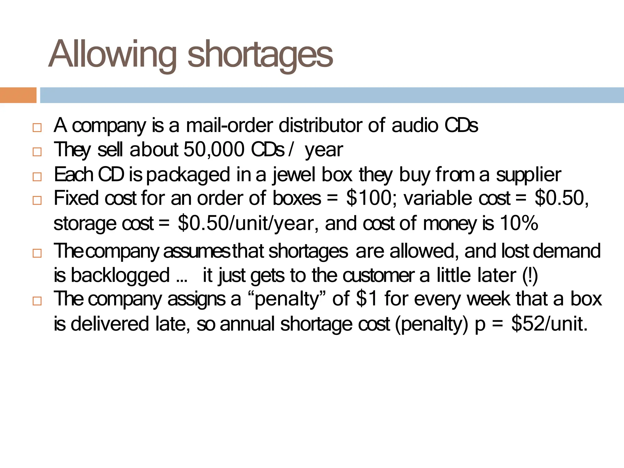
Allowing shortages

57. Production Order Quantity Model
1. Used when inventory buildsup over a period
of time after an order isplaced
2. Used when units are produced and sold
simultaneously
Inventory
level
Time
Part of inventorycycleduring which
production (and usage) istaking place
Demand part of cycle with
no production (only usage)
t
Maximu
m
inventory

58. Production Order Quantity Model
Q =Number of pieces per order
H =Holding cost per unit per year
p = Daily production rate
d = Daily demand/usage rate
t =Length of the production run in days
= (Average inventory level) x
Annual inventory
holding cost
Holding cost
per unit per year
= (Maximum inventory level)/2
Average
inventory level
= –
Maximum
inventory level
Total items produced
during the production
run
Total items used
during the
production run
= pt – dt

59. Production Order Quantity Model
Q =Number of pieces per order
H =Holding cost per unit per year
p = Daily production rate
d = Daily demand/usage rate
t =Length of the production run in days
= – Total used during
the production run
Maximum
inventory level
Total produced during
the production run
= pt – dt
However, Q = total produced = pt ; thus t = Q/p
Maximum
inventory level = p
p
– d
Q
= Q 1 – d
Q
p p
Holding cost = (H) = 1 – H
d
p
Q
2
Maximum inventory level
2

60. Production Order Quantity Model
Q =Number of pieces per order
H =Holding cost per unit per year
p = Daily production rate
d = Daily demand/usage rate
t =Length of the production run in days
Setup cost = (D / Q)S
1
2
Holding cost = HQ 1 d p


 
D
Q
1
2
S  HQ 1 d p


 
2
Q 
2DS
H1d p
 
p
Q*

2DS
H1d p
 
Q*

2DS
H
Remember,
with no
production
taking place

61. Production Order Quantity Example
D =1,000 units
S =$10
H =$0.50 per unit per year
p = 8 units per day
d = 4 units per day
Qp
*

2DS
H1d p
2(1,000)(10)
Qp
*

0.501(4 8)

20,000
0.50(1 2)
 80,000
 282.8 units, or 283 units

62. Production Order Quantity Model
When annual data are used the equation becomes
Note:
d = 4 = =
D
Number of days the plant is in operation
1,000
250
p
Q*

2DS
Annual demand rate
 
H 
1
Annual production rate

 

63. Probabilistic Models and Safety Stock

64. Probabilistic Models and
Safety Stock
▶ Demand isoften UNCERTAIN
▶ The problem appears when there isLEADTIME, L
▶ We have to set two parameters that define our
ordering policy: R
eorder P
oint (ROP) and Safety Stock
(ss)
▶ You reorder when your inventory fallson or below ROP
▶ Use safety stock to achieve a desired service level and
avoid stockouts
ROP = d x L + ss
ExpectedAnnual stockout costs = (expected units short/ cycle)
x the stockout cost/unit x the number of orders per year

65. Safety Stock Example
NUMBER OF UNITS
(d X L)
PROBABILITY
30 .2
40 .2
Current ROP  50 .3
60 .2
70 .1
1.0
Current policy:
ROP= 50 units
Orders per year = 6
Stockout cost = $40 / unit
Carrying cost = $5 / unit / year
Probability distribution for inventory demand during lead time
How much safety stock should we keep and added to 50 (current ROP)?

66. Safety Stock Example
ROP= 50 units
Orders /year = 6
Stockout cost = $40 /unit
Carrying cost = $5 /unit/ year
SAFE
TY
STOCK
ADDITIONAL
HOLDING
COST
STOCKOUT COST
TOTA
L
COST
20 (20)($5) = $100 $0 $100
10 (10)($5) = $ 50 (10)(.1)($40)(6) = $240 $290
0 $ 0 (10)(.2)($40)(6) + (20)(.1)($40)(6) = $960 $960
A safety stock of 20 units gives the lowest total cost
ROP= 50 + 20 = 70 frames

67. Probabilistic Demand
Use prescribed service levelsto set safety stock
when the cost of stockouts cannot be determined
ROP= demand during lead time + ZdLT
Where:
Z = Number of standard deviations
dLT = Standard deviation of demand during lead time

68. Safety
stock
Probability of
no stockout
95% of the time
Mean
demand
350
ROP = ? kits Quantity
Number of
standard deviations
0 z
Risk of a stockout
(5% of area of
normal curve)
Probabilistic Demand

69.  = Average demand = 350 kits
dLT = Standard deviation of demand during lead time
= 10 kits
Z = 5% stockout policy (service level = 95%)
Using Normal distribution tables, for an area
under the curve of 95%, the Z = 1.65
Safety stock = ZdLT = 1.65(10) = 16.5 kits
Reorder point = Expected demand during lead time +
Safety stock
= 350 kits + 16.5 kits of safety stock
= 366.5 or 367 kits
Probabilistic Demand

70. Safety stock 16.5 units
ROP 
Place
order
Probabilistic Demand
Inventory
level
Time
0
Normal distribution probability of
demand during lead time
Expected demand during lead time (350 kits)
Minimumdemand during lead time
Maximum demand during lead time
Mean demand during lead time
ROP = 350 + safety stock of 16.5 = 366.5
order
Lead Receive
time

71. Other Probabilistic Models
▶ When data on demand during lead time is not
available, there are other models available
1. When demand is variable and lead time is
constant
2. When lead time is variable and demand is
constant
3. When both demand and lead time are variable

72. Other Probabilistic Models:
Variable demand, constant lead time
Demand is variable and lead time is constant
ROP = (Average daily demand
x Lead time in days) + ZdLT
where dLT = d Lead time
d = standard deviation of demand per day

73. Average daily demand (normally distributed) = 15
Lead time in days (constant) = 2
Standard deviation of daily demand = 5
Service level = 90%
Z for 90% = 1.28
From Appendix I
ROP = (15 units x 2 days) + ZdLT
= 30 + 1.28(5)( 2)
= 30 + 9.02 = 39.02 ≈ 39
Safety stock is about 9 computers
Other Probabilistic Models:
Variable demand, constant lead time

74. ROP = (Daily demand x Average lead time in days)
+ Z x (Daily demand) x LT
where LT = Standard deviation of lead time in days
Other Probabilistic Models:
Constant demand, variable lead time

75. Daily demand (constant) = 10
Average lead time = 6 days
Standard deviation of lead time = LT = 1
Service level = 98%, so Z (fromAppendix I) = 2.055
ROP = (10 units x 6 days) + 2.055(10 units)(1)
= 60 + 20.55 = 80.55
Reorder point is about 81 cameras
Other Probabilistic Models:
Constant demand, variable lead time

76. ROP = (Average daily demand x Average lead time)
+ ZdLT
where d= Standard deviation of demand per day
LT= Standard deviation of lead time in days
dLT= (Average lead time x  2)
d
+ (Average daily demand)2
LT
Other Probabilistic Models:
Variable demand, variable lead time

77. Average daily demand (normally distributed) = 150
Standard deviation = d = 16
Average lead time 5 days (normally distributed)
Standard deviation = LT = 1 day
Service level = 95%, so Z = 1.65 (from Normal tables)
ROP  (150 packs5 days)1.65dLT
dLT  5 days162
1502
12
 525622,5001
 1,28022,500 23,780 154
ROP  (1505)1.65(154)  750254 1,004 packs
Other Probabilistic Models:
Variable demand, variable lead time

78. Inventory Control Systems

79. Inventory Control Systems
 Continuousreview (Q) system
🞑 R
eorder point system (ROP) and fixed order
quantity system
🞑 For independent demand items (i.i.d.)
🞑 T
racksinventory position (IP)
🞑 Includesscheduledreceipts (SR),on-handinventory
(OH), and back orders (BO)
Inventory position = On-hand inventory + Scheduled receipts
– Backorders
IP = OH + SR – BO

80. Selecting the Reorder Point
Time
On-hand
inventory
TBO TBO
L L
TBO
L
Order
placed
Order
placed
Order
placed
IP IP
IP
R
Q Q
Q
OH OH
OH
Order
received
Order
received
Order
received
Order
received
Q System When Demand and Lead Time Are Constant and Certain

81. Continuous R
eview Systems
The on-hand inventory isonly 10 units, and the
reorder point R is100. There are no
backorders, but there is one open order for 200 units.
Should a new order be placed?
SOLUTION
IP = OH + SR – BO = 10 + 200 – 0 = 210
R = 100
Decision: Do not place a new order

82. Continuous R
eview Systems
Reorder Point Level:
Assuming that the demand rate per period and the
lead time are constant,thelevel of inventory at
which a new order is placed (reorder point) can be
calculated asfollows:
R = dL
Where
d = demand rate per period
L = lead time
R
emember: The order quantity Q isthe EOQ!

83. Continuous R
eview Systems
EXAMPLE4
Demand for chicken soup at a supermarket is always 25 cases
a day and the lead time is always 4 days. The shelves were just
restockedwith chickensoup,leaving an on-hand inventory of
only 10 cases.No backorders currently exist, but there isone
open order in the pipeline for 200 cases. What is the inventory
position? Should a new order be placed?
SOLUTION
R =Total demand during lead time = (25)(4) = 100 cases
IP = OH + SR – BO
= 10 + 200 – 0 = 210 cases
Decision: Do not place a new order

84. Continuous R
eview Systems
 Selecting the reorder point with variable demand
and constant lead time
Reorder point = Average demand during lead time
+ Safety stock
= dL + safety stock
where
d = average demand per week (or day or months)
L = constant lead time in weeks (or days or months)

85. Continuous R
eview
Systems (uncertain
demand)
Time
On-hand
inventory
TBO1 TBO2 TBO3
L1 L2 L3
R
Order
received
Q
Order
placed
Order
placed
IP
Order
received
IP
Q
Order
placed
Q
Order
received
Order
received
0
IP
Q System When Demand Is Uncertain

86. How to determine the R
eorder P
oint
1. Choose an appropriate service-level policy
🞑 Select service level or cycle service level
🞑 Protection interval
2. Determine the demand during lead time
probability distribution
3. Determine the safety stock and reorder point
levels

87. Demand During Lead Time
 Specify mean d and standard deviation σd for the demand
(typically these values are given)
 Calculate standard deviation of demand during lead time L
σdLT =
σd L = σd L
2
 Then, the safety stock and reorder point are
Safety stock = zσdLT
where
z =number of standard deviations needed to achieve the
cycle-service level (found from tables)
σdLT = stand deviation of demand during lead time
Reorder point = R = dL + safety stock

88. Demand During Lead Time
Average
demand
during
lead time
Cycle-service level = 85%
Probability of stockout
(1.0 – 0.85 = 0.15)
R
zσdLT
Finding Safety Stock with a Normal Probability Distribution for an 85 Percent
Cycle-Service Level

89. R
eorder P
oint for Variable Demand
EXAMPLE5
Let usreturn to the bird feeder in Example 2.
The EOQ is75 units.
Suppose that the average demand is 18 units per week with
a standard deviation of 5 units.
The lead time isconstant at two weeks.
Determine the safety stock and reorder point if
management wants a 90 percent cycle-service level.

90. R
eorder P
oint for Variable Demand
SOLUTION
In this case, σd = 5, d = 18 units, and L = 2 weeks, so
σdLT = σd L = 5 2 = 7.07. Consult the body of the table in the
Normal Distribution appendix for 0.9000, which corresponds to
a 90 percent cycle-service level. The closest number is 0.8997,
which corresponds to 1.2 in the row heading and 0.08 in the
column heading. Adding these values gives a z value of 1.28.
With this information, we calculate the safety stock and reorder
point as follows:
Safety stock = zσdLT = 1.28(7.07) = 9.05 or 9 units
Reorder point = dL + Safety stock = 2(18) + 9 = 45 units

91. R
eorder P
oint for Variable Demand
EXAMPLE6
Suppose that the demand during lead time is normally distributed with an
average of 85 and σdLT = 40. Find the safety stock, and reorder point R,
for a 95 and 85 percent cycle-service level.
SOLUTION
Safety stock = zσdLT = 1.645(40) = 65.8 or 66 units
R = Average demand during lead time + Safety stock
R = 85 + 66 = 151 units
Find the safety stock, and reorder point R, for an 85 percent
cycle-service level.
Safety stock = zσdLT = 1.04(40) = 41.6 or 42 units
R = Average demand during lead time + Safety stock
R = 85 + 42 = 127 units

92. R
eorder P
oint for Variable Demand &
Variable Lead Time
σdLT =
Lσd + d σLT
2 2 2
 Often the case that both are variable
 The equations are more complicated
Safety stock = zσdLT
R =(Average weekly demand  Average lead time)
+ Safety stock
= dL + Safety stock
where
d =Average weekly (or daily or monthly) demand
L =Average lead time
σd = Standard deviation of weekly (or daily or monthly) demand
σLT = Standard deviation of the lead time

93. R
eorder P
oint for Variable
Demand & Variable Lead Time
EXAMPLE7
The Office Supply Shop estimates that the average demand for
a popular ball-point pen is12,000 pens per week with a
standard deviation of 3,000 pens. The current inventory policy
callsfor replenishment orders of 156,000 pens. The average
lead time from the distributor is5 weeks, with a standard
deviation of 2 weeks. If management wants a 95 percent cycle-
service level, what should the reorder point be?

94. R
eorder P
oint for Variable
Demand & Variable Lead Time
SOLUTION
We have d = 12,000 pens, σd = 3,000 pens, L = 5 weeks,
and σLT = 2 weeks
σdLT =
Lσd + d σLT = (5)(3,000) + (12,000) (2)
2 2 2 2 2 2
= 24,919.87 pens
From the Normal Distribution appendix for 0.9500, the
appropriate z value = 1.65. We calculate the safety stock and
reorder point as follows:
Safety stock = zσdLT = (1.65)(24,919.87)
= 41,117.79 or 41,118 pens
Reorder point = dL + Safety stock = (12,000)(5) + 41.118
= 101,118 pens

95. R
eorder P
oint for Variable
Demand & Variable Lead Time
EXAMPLE8
Grey Wolf lodge isa popular 500-room hotel in the North
Woods. Managers need to keep close tabson all of the room
service items,including a special pint-scented bar soap. The
daily demand for the soap is275 bars, with a standard
deviation of 30 bars. Ordering costis$10 and theinventory
holding cost is $0.30/bar/year. The lead time from the supplier
is5 days, with a standard deviation of 1 day. The lodge is
open 365 days a year.
What should the reorder point be for the bar of soap if
management wants to have a 99 percent cycle-service?

96. R
eorder P
oint for Variable
Demand & Variable Lead Time
SOLUTION
d =275 bars
L =5 days
σd = 30 bars
σLT = 1 day
Lσd + d σLT = 283.06 bars
2 2 2
σdLT =
From the Normal Distribution appendix for 0.9900, z = 2.33.
We calculate the safety stock and reorder point as follows;
Safety stock = zσdLT = (2.33)(283.06) = 659.53 or 660 bars
Reorder point + safety stock = dL + safety stock
= (275)(5) + 660 = 2,035 bars

97. P
eriodic R
eview (or fixed period)
System (P)
 Fixed interval reorder system or periodic reorder system
 Four of the original EOQ assumptions maintained
🞑 No constraints are placed on lot size
🞑 Holding and ordering costs
🞑 Independent demand
🞑 Lead timesare certain
 Order is placed to bring the inventory position up to the target
inventory level, T, when the predetermined time, P, has elapsed
▶Only relevant costs are ordering and holding
▶Lead times are known and constant
▶Items are independent of one another

98. P
eriodic R
eview Systems
On-hand
inventory
Q1
Q2
Target quantity (T)
P
Q3
Q4
P
P
Time

99. ▶ Inventory is only counted at each review
period
▶ May be scheduled at convenient times
▶ Appropriate in routine situations
▶ May result in stockouts between periods
▶ May require increased safety stock
P
eriodic R
eview Systems

100. P
eriodic R
eview System (P)
P P
T
L L L Time
On-hand
inventory
IP1
IP3
IP2
Order
placed
Order
placed
Order
received
Order
received
Order
received
IP IP
IP
OH OH
Q1
Q2
Q3
Protection interval
P System When Demand Is Uncertain

101. How Much to Order in a P System
EXAMPLE9
Adistribution center has a backorder for five 36-inch color TV sets.
No inventory iscurrently on hand, and now isthe time to review. How
many should be reordered if T = 400 and no receipts are scheduled?
SOLUTION
IP = OH + SR – BO
= 0 + 0 – 5 = –5 sets
T – IP = 400 – (–5) = 405 sets
That is, 405 sets must be ordered to bring the inventory
position up to T sets.

102. How Much to Order in a P System
EXAMPLE10
The on-hand inventory is10 units, and T is400. There are no
back orders, but one scheduled receipt of 200 units. Now is the
time to review. How much should be reordered?
SOLUTION
IP = OH + SR – BO
= 10 + 200 – 0 = 210
T – IP = 400 – 210 = 190
The decision is to order 190 units

103. P
eriodic R
eview System
 Selecting the time between reviews, choosing P and T
 Selecting Twhen demand isvariable and lead time is
constant
IP covers demand over a protection interval of P + L
The average demand during the protection interval is
d(P + L), or
T = d(P + L) + safety stock for protection interval
Safety stock = zσP + L , where σP + L = d P L

104. Calculating P and T
EXAMPLE11
Again, let usreturn to the bird feeder example. Recall that
demand for the bird feeder isnormally distributed with a mean
of 18 unitsper weekand a standard deviation inweekly
demandof 5 units.Thelead timeis2 weeks,and thebusiness
operates 52 weeks per year. The Q system developed in
Example5 called for anEOQof 75 units and a safety stock of
9 unitsfor a cycle-service level of 90 percent. What isthe
equivalent P system?Answersare to be rounded to thenearest
integer.

105. Calculating P and T
SOLUTION
We first define D and thenP. Here,P isthetime between
reviews, expressed in weeks because the data are expressed
asdemand per week:
D = (18 units/week)(52 weeks/year) = 936 units
P =
EOQ
(52) = 75 (52) = 4.2 or 4 weeks
D 936
With d = 18 units per week, an alternative approach is to calculate P
by dividing the EOQ by d to get 75/18 = 4.2 or 4 weeks. Either way,
we would review the bird feeder inventory every 4 weeks.

106. Calculating P and T
We now find the standard deviation of demand over the protection
interval (P + L) = 6:
Before calculating T, we also need a z value. For a 90 percent
cycle-service level z = 1.28. The safety stock becomes
Safety stock = zσP + L = 1.28(12.25) = 15.68 or 16 units
We now solve for T:
T = Average demand during the protection interval + Safety stock
= d(P + L) + safety stock
= (18 units/week)(6 weeks) + 16 units = 124 units
P L  5 6 12.25 units
PL d

107. Comparative Advantages
 Primary advantages of P systems
🞑 Convenient
🞑 Orders canbe combined
🞑 Only need to know IPwhen review ismade
 Primary advantages of Q systems
🞑 Review frequency may be individualized
🞑 Fixed lot sizes canresult in quantity discounts
🞑 Lower safety stocks

108. Single Period Model

109. Single-Period Model
▶ Only one order is placed for a product
▶ Units have little or no value at the end of the
sales period
▶ Newsboy problem 1:
▶ Demand = 500 papers/day, σ = 100 paper
▶ Cost to newsboy = 10c, Sales price = 30c
▶ How many papers should he order?

110. The newsboy problem
▶ If he sellsa paper, he makes a profit = 20c
▶ If he doesn’t sell a paper he makes a loss= 10c
▶ If he orders x papers, on the i-th paper he
makes an expected profit:
▶ E(Profit)i = 20p – 10(1-p), where p=sale of i-th paper
▶ Breakeven occurs when the Expected profit = 0
▶ So, 20p – 10(1-p) = 0, and therefore p* = 1/3
▶ By looking at the Normal tables, Z = .431
p
1-p
 = 500
Optimal stocking level

111. The newsboy problem
▶ Therefore:
▶ Z = .431 = (X*-μ)/σ = (X*-500)/100
▶ X* = 543
1-p
 = 500
Optimal stocking level

112. A small variation
▶ Assume that he can return the paper, if unsold for 5c each
▶ E(Profit)i= 20p – 5(1-p), where p=sale of i-th paper
▶ Breakeven occurs when the Expected profit = 0
▶ So, 20p – 5(1-p) = 0, and therefore p* = 1/5
▶ By looking at the Normal tables, Z = .842
▶ Then, X* = 584
▶ In general, if MR= Marginal Return and ML = Marginal
Loss, then p MR- (1-p) ML = 0
▶ p* = ML/(MR+ML)

113. Using Simulation for stochastic inventory
management

114. What is Simulation ?
Simulation isa model – computer code – “imitating”
the operation of a real systemin the computer.
It consistsof:
a)A set of variables representing the basic features
of the real systemand
b)A set of logical commands in the computer that
modify these features as a function of time in
accordance with the rules (logical of physical)
regulating the real system.

115.  Thecapacity to "advance time" throughtheuseof a
simulation build-in clock that monitors and the events while
stepping up real time
 Thecapacity of drawing samplesthroughthecreation of
artificial observationsthat behave "like" random events in
the real system
🞑 a) Creation of random numbers (independent & uniformly
distributed) by the computer (according to an internal algorithm -
function)
🞑 Conversion in the observations’ distribution
Main Features of a Simulation
System

116. Examples of applications
Very important tool for
 Service management - Analysis of queuing systems
 Business Process Reengineering
 Strategic planning
 Financial planning
 Industrial design (e.g. chemical plants)
 Short term production planning
 Quality and reliability control,
 Training – business games, etc

117. Let us suppose that the weekly demand of a
product can take the following values with the
respective probabilities:
Creating random numbers according
to a probability distribution
Demand (D)
Probability of Demand
P(D)
Cumulative Distribution of
Demand F(D)
1,000 0.20 0.20
1,500 0.10 0.30
2,000 0.30 0.60
2,500 0.25 0.85
3,000 0.15 1.00

118. D1
D2
.,30
0.20
0.60
1.00
0.85
1.000 1,500 2,000 2,500 3,000
R1
R2
The cumulative probability
distribution F

119. Example
Week
Unif.
Random
Number
Week's
Deman
d
1 32 2,000
2 8 1,000
3 46 2,000
4 92 3,000
5 69 2,500
6 71 2,500
7 29 1,500
8 46 2,000
9 80 2,500
10 14 1,000
Demand (D)
Cumulative Distribution of
Demand F(D)
1,000 0.20
1,500 0.30
2,000 0.60
2,500 0.85
3,000 1.00
Remember, the
Cumulative
Distribution F
Createa"demand
series“ corresponding
totherandomnumbers
generated

120. Using Simulation to define
an Inventory Policy
 Assume that a company is interested to implement an (s, S)
ordering policy. Determine values of s and S:
 s = Safety stock S = Order-up-to quantity
Inventory Behavior (s = 200, S = 700)
800
700
600
500
400
300
200
100
0
1 2 3 4 5 6 7 8 9 10 11 12 13
Weeks
Demand
Inventory
levels
Series2
Series1

121. Demand (D)
Probability of Demand
P(D)
Cumulative Distribution of
Demand F(D)
1,000 0.20 0.20
1,500 0.10 0.30
2,000 0.30 0.60
2,500 0.25 0.85
3,000 0.15 1.00
Key assumptions:
• When < the safety stock s, order up to the reorder point S
• When short, make emergency order for quantity short
• Normal ordering cost = 200 + 10 • quantity
• Emergency ordering cost = 500 + 15 • quantity
• Leftover inventory cost = 3 • quantity
Application to our problem

122. Flow chart
STARTOF SIMULATION
 Define initial conditions
 Define strategy parameters s, S
Next week, t = t+1
Simulation complete? STOP
 Compute Average
Weekly cost
Compute other
performance criteria
Need to order?
 Order amount S-I
 Update inventory to S
 P
ay ordering cost
 Update total cost
Create demand D for this week
Isdemand satisfied?
 Update inventory level
 P
ay holding cost
 Update total cost
 Place emergency order
 Update inventory level
 P
ay emergency cost
 Update total cost

123. Manual Simulation of Inventory
System
 Assume: s = 1,500 and S = 2,500
Week
Starting
Inventor
y
Need
to
order?
Size
of
order
Availabl
e
inventor
y
Week's
Deman
d
Emergenc
y
order?
Size of
emerg.
order
Ending
Inventor
y
Weekl
y
Cost
1 2,000 no 0 2,000 2,000 no 0 0 0
2 0 yes 2,500 2,500 2,000 no 0 500 26,700
3 500 yes 2,000 2,500 3,000 yes 500 0 30,500
4 0 yes 2,500 2,500 1,000 no 0 1,500 29,700
5 1,500 yes 1,000 2,500 2,500 no 0 0 10,200
6 0 yes 2,500 2,500 2,500 no 0 0 25,200
7 0 yes 2,500 2,500 3,000 yes 500 0 38,000
8 0 yes 2,500 2,500 1,500 no 0 1,000 28,200
9 1,000 yes 1,500 2,500 2,000 no 0 500 16,700
10 500 yes 2,000 2,500 2,500 no 0 0 20,200
Average 389 always 2,111 2,500 2,200 20% 500 389 25,044