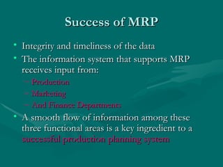
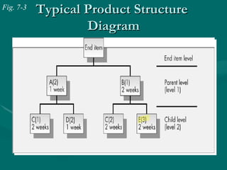
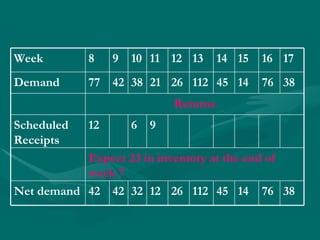
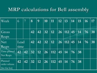
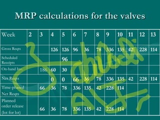
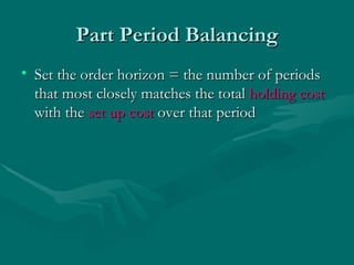
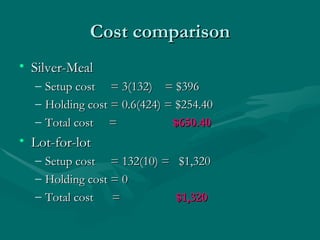
The document discusses push and pull production control systems. A push system like MRP initiates production based on forecasts, while a pull system like JIT initiates production based on current demand. MRP involves gathering demand data, determining planned order releases using explosion calculus, and developing shop floor schedules. Lot sizing algorithms aim to balance setup and holding costs. Capacity constraints and improvement steps can further optimize production planning.

1. Chapter 7 Push and Pull Production Control Systems MRP and JIT

2. Push and Pull Control Systems A Push System (MRP) initiates production in anticipation of future demand Incorporates forecasts of future demand A Pull System initiates production as a reaction to present demand (JIT) Initiates production as a reaction of … demand

3. Difference between MRP and JIT MRP: Determine lot sizes based on future demand forecasts JIT Reduce lot sizes to eliminate waste and unnecessary buildups of inventory

4. MRP Basics Production Plan M aster P roduction S chedule (MPS) MRP system Job shop Schedule At the heart of the production plan are the demand forecasts of end items End item: Components Raw materials Figure 7-1

5. Schematic of the Productive System Fig. 7-1

6. Production Plan MPS : specification of the exact amounts and timing of production of each of the end items MRP is the means by which MPS is broken down into a detailed schedule of production for each component that comprises an end item MRP results are translated into specific shop floor schedules

7. Data sources for determining the MPS Firm customer orders Forecasts of future demand by item Safety stock requirements Seasonal plans Internal orders from other parts of the organization

8. Success of MRP Integrity and timeliness of the data The information system that supports MRP receives input from: Production Marketing And Finance Departments A smooth flow of information among these three functional areas is a key ingredient to a successful production planning system

9. Major phases of the control system Phase 1: Gathering and coordinating of the information require to develop the MPS Phase 2: Determination of planned order releases using MRP Phase 3: Development of detailed shop floor schedules and resource requirements from the MRP planned order releases

10. The Three Major Control Phases of the Productive System Fig. 7-2

11. Explosion Calculus Bill of Material (BOM) explosion Set of rules by which gross requirements at one level of the product structure are translated into a production schedule at that level and requirements at lower levels At the heart of the MRP system is the product structure (figure 7-3): The method is best illustrated with an example:

12. Typical Product Structure Diagram Fig. 7-3

13. Trumpet and Subassemblies Fig. 7-4

14. Product Structure Diagram for Harmon Trumpet Fig. 7-5

15. Indented BOM 1 Trumpet 1 Bell assembly 1 Valve assembly 3 slide assemblies 3 valves

16. 38 76 14 45 112 26 12 32 42 42 Net demand Expect 23 in inventory at the end of week 7 9 6 12 Scheduled Receipts Returns 38 76 14 45 112 26 21 38 42 77 Demand 17 16 15 14 13 12 11 10 9 8 Week

17. MRP calculations for Bell assembly 38 76 14 45 112 26 12 32 42 42 Planned order release (lot for lot) 38 76 14 45 112 26 12 32 42 42 Time-phased Net Reqts 38 76 14 45 112 26 12 32 42 42 Lead time Net Reqts 38 76 14 45 112 26 12 32 42 42 Gross Reqts 17 16 15 14 13 12 11 10 9 8 7 6 Week

18. MRP calculations for the valves 30 60 186 On-hand Inv. 96 Scheduled Receipts 114 228 42 135 336 78 36 66 Planned order release (lot for lot) 114 228 42 135 336 78 36 66 Time-phased Net Reqts 114 228 42 135 336 78 36 66 0 0 Net Reqts 114 228 42 135 336 78 36 96 126 126 Gross Reqts 13 12 11 10 9 8 7 6 5 4 3 2 Week

19. Incorporating the lot-sizing algorithms into the explosion calculus ___________________________________________ Week 4 5 6 7 8 9 10 11 12 13 Time-phased 42 42 32 12 26 112 45 14 76 38 Net Reqts _____________________________________________________________________________ Valve casing assembly

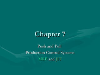
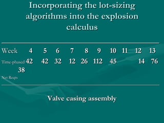
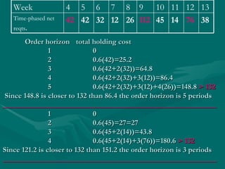
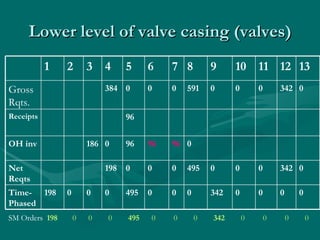
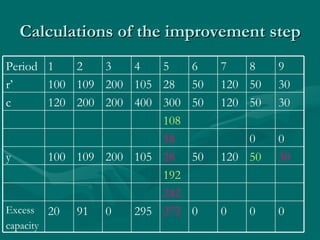
20. Starting in week 4 C(1)=132 C(2)=[132+0.6(42)]/2=78.6 C(3)=[132+0.6(42+2(32))]/3=65.2 C(4)=[132+0.6(42+2(32)+3(12))]/4=54.3 C(5)=[132+0.6(42+2(32)+3(12)+4(26))]/5=55.92  y 4 = 42+42+32+12=128 38 76 14 45 112 26 12 32 42 42 Time-phased net reqts . 13 12 11 10 9 8 7 6 5 4 Week

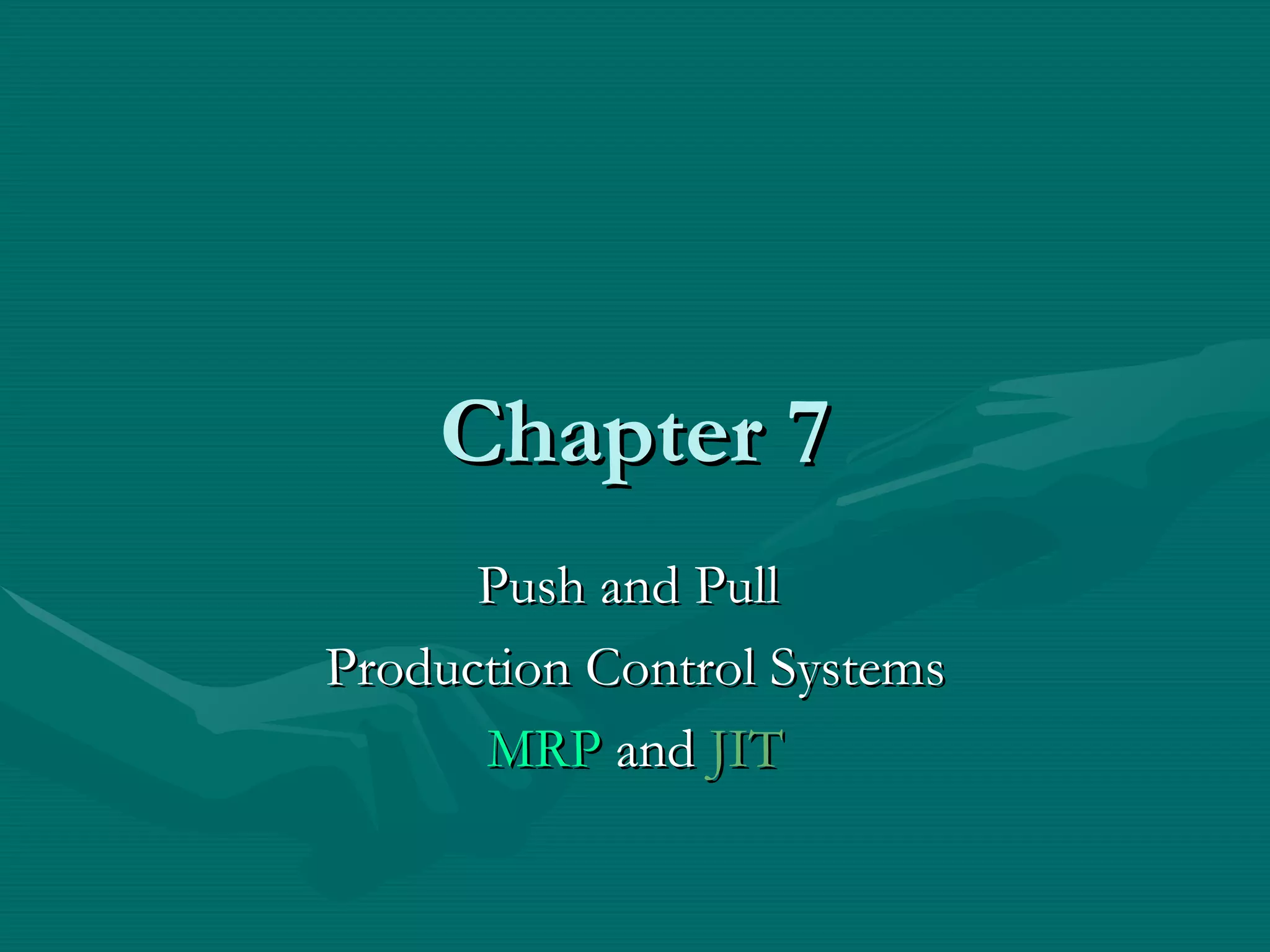
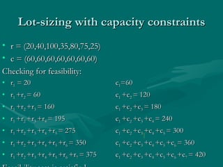
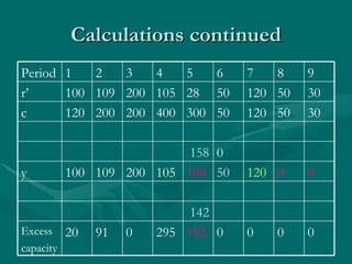
21. Starting in week 8: C(1)=132 C(2)=[132+0.6(112)]/2=99.6 C(3)=[112+0.6(112+2(45))]/3=84.4 C(4)=[112+0.6(112+2(45)+3(14))]/4=69.6 C(5)=[112+0.6(112+2(45)+3(14)+4(76))]/5=92.16  y 8 = 26+112+45+14=197 38 76 14 45 112 26 12 32 42 42 Time-phased net reqts. 13 12 11 10 9 8 7 6 5 4 Week

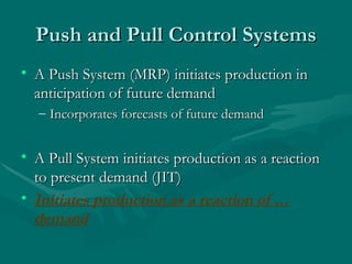
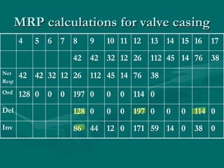
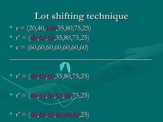
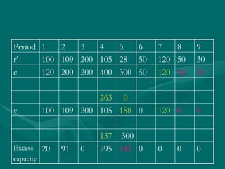
22. Starting in week 12: C(1)=132 C(2)=[132+0.6(38)]/2=77.4  y 12 = 76+38=114 Week 4 5 6 7 8 9 10 11 12 13 Pon 128 0 0 0 197 0 0 0 114 0 38 76 14 45 112 26 12 32 42 42 Time-phased net reqts. 13 12 11 10 9 8 7 6 5 4 Week

23. Part Period Balancing Set the order horizon = the number of periods that most closely matches the total holding cost with the set up cost over that period

24. Order horizon total holding cost 1 0 2 0.6(42)=25.2 3 0.6(42+2(32))=64.8 4 0.6(42+2(32)+3(12))=86.4 5 0.6(42+2(32)+3(12)+4(26))=148.8 > 132 Since 148.8 is closer to 132 than 86.4 the order horizon is 5 periods _________________________________________________________ 1 0 2 0.6(45)=27=27 3 0.6(45+2(14))=43.8 4 0.6(45+2(14)+3(76))=180.6 > 132 Since 121.2 is closer to 132 than 151.2 the order horizon is 3 periods _________________________________________________________ 38 76 14 45 112 26 12 32 42 42 Time-phased net reqts . 13 12 11 10 9 8 7 6 5 4 Week

25. MRP calculations for valve casing Inv Del Ord Net Reqt 0 38 0 14 59 171 0 12 44 86 128 42 4 12 0 114 0 0 0 197 0 0 0 128 0 114 0 0 0 197 0 0 0 38 76 14 45 112 26 32 42 38 76 14 45 112 26 12 32 42 42 17 16 15 14 13 12 11 10 9 8 7 6 5

26. Cost comparison Silver-Meal Setup cost = 3(132) = $396 Holding cost = 0.6(424) = $254.40 Total cost = $650.40 Lot-for-lot Setup cost = 132(10) = $1,320 Holding cost = 0 Total cost = $1,320

27. Lower level of valve casing (valves) SM Orders 198 0 0 0 495 0 0 0 342 0 0 0 0 Time-Phased Net Reqts OH inv Receipts Gross Rqts. 0 0 0 0 342 0 0 0 495 0 0 0 198 1 0 342 0 0 0 495 0 0 0 198 0 96 96 96 0 186 96 0 342 0 0 0 591 0 0 0 384 13 12 11 10 9 8 7 6 5 4 3 2

28. Lot-sizing with capacity constraints r = (20,40,100,35,80,75,25) c = (60,60,60,60,60,60,60) Checking for feasibility: r 1 = 20 c 1 =60 r 1 +r 2 = 60 c 1 +c 2 = 120 r 1 +r 2 +r 3 = 160 c 1 +c 2 +c 3 = 180 r 1 +r 2 +r 3 +r 4 = 195 c 1 +c 2 +c 3 +c 4 = 240 r 1 +r 2 +r 3 +r 4 +r 5 = 275 c 1 +c 2 +c 3 +c 4 +c 5 = 300 r 1 +r 2 +r 3 +r 4 +r 5 +r 6 = 350 c 1 +c 2 +c 3 +c 4 +c 5 +c 6 = 360 r 1 +r 2 +r 3 +r 4 +r 5 +r 6 +r 7 = 375 c 1 +c 2 +c 3 +c 4 +c 5 +c 6 +c 7 = 420 Feasibility test is satisfied

29. Lot shifting technique r = (20,40, 100 ,35,80,75,25) r’ = ( 40 , 60 , 60 ,35,80,75,25) c = (60,60,60,60,60,60,60) _______________________________________ r’ = ( 40 , 60 , 60 ,35,80,75,25) r’ = ( 40 , 60 , 60 , 55 , 60 ,75,25) r’ = ( 50 , 60 , 60 , 60,60,60 ,25)

30. The improvement step K=450 and h =2 r = (100, 79, 230, 105, 3, 10, 99, 126,40) c = (120, 200, 200, 400, 300, 50, 120, 50, 30) 0 0 0 0 272 295 0 91 20 Excess capacity 30 50 120 50 28 105 200 109 100 y 30 50 120 50 300 400 200 200 120 c 30 50 120 50 28 105 200 109 100 r’ 9 8 7 6 5 4 3 2 1 r’

31. Calculations of the improvement step 0 0 0 0 272 295 0 91 20 Excess capacity 242 192 30 50 120 50 28 105 200 109 100 y 0 0 58 108 30 50 120 50 300 400 200 200 120 c 30 50 120 50 28 105 200 109 100 r’ 9 8 7 6 5 4 3 2 1 Period

32. Calculations continued 0 0 0 0 192 295 0 91 20 Excess capacity 142 0 0 120 50 108 105 200 109 100 y 0 158 30 50 120 50 300 400 200 200 120 c 30 50 120 50 28 105 200 109 100 r’ 9 8 7 6 5 4 3 2 1 Period

33. 0 0 0 0 142 295 0 91 20 Excess capacity 300 137 0 0 120 0 158 105 200 109 100 y 0 263 30 50 120 50 300 400 200 200 120 c 30 50 120 50 28 105 200 109 100 r’ 9 8 7 6 5 4 3 2 1 Period

34. 0 0 0 0 300 137 0 91 20 Excess capacity 0 0 120 0 0 263 200 109 100 y 30 50 120 50 300 400 200 200 120 c 30 50 120 50 28 105 200 109 100 r’ 9 8 7 6 5 4 3 2 1 Period

35. Cost comparison Initial solution Holding cost = 2 (0+30+0+0+25+65+86+10)=432 Set up cost = 9 x 450 = 4,050 Total Cost = 432 + 4,050 = 4,482 Improved solution Holding cost = 2 (0+30+0+158+155+145+166+40+0) = 2 x 694 = 1,388 Set up cost = 5 x 450 = 2,250 Total cost = 1,388 + 2,250 = 3,638