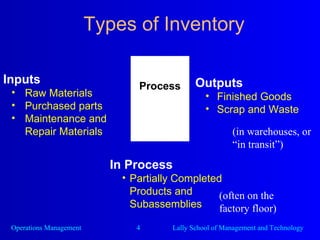
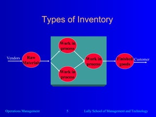
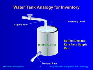
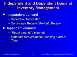
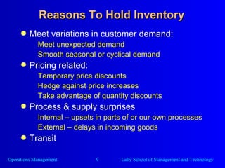
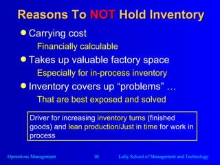
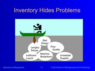
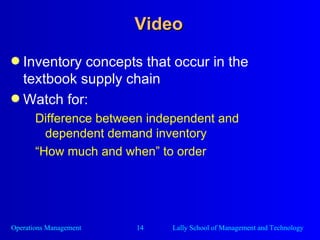
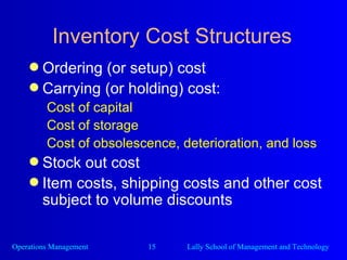
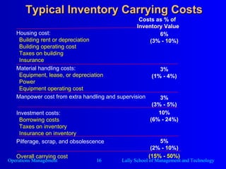
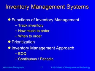
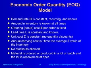
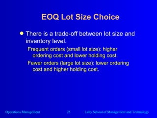
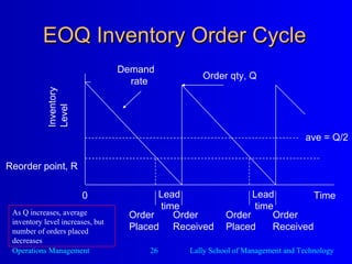
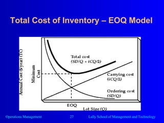
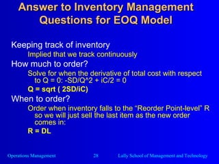
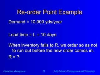
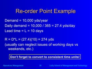
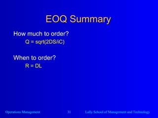
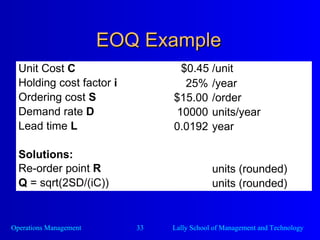
The document discusses inventory management concepts. It defines types of inventory like raw materials, work in process, and finished goods. It explains the difference between independent and dependent demand and how they are managed. There are reasons to hold inventory, like meeting demand variations, and reasons not to hold too much like carrying costs. The Economic Order Quantity (EOQ) model is introduced for determining how much and when to order to minimize total inventory costs based on demand, ordering costs, carrying costs, and lead times. Managers must find the optimal balance of ordering and carrying costs.

1. Inventory

2. Inventory - I Items from last class What is inventory Inventory Video Inventory Cost Structure Basic Ideas for Managing Independent Demand Inventory Economic Order Quantity Exercise

3. Inventory Definition A stock of items held to meet future demand Question: Goods vs Services?

4. Types of Inventory Inputs Raw Materials Purchased parts Maintenance and Repair Materials Outputs Finished Goods Scrap and Waste Process In Process Partially Completed Products and Subassemblies (in warehouses, or “in transit”) (often on the factory floor)

5. Types of Inventory Work in process Work in process Work in process Finished goods Raw Materials Vendors Customer

6. Water Tank Analogy for Inventory Supply Rate Inventory Level Demand Rate Inventory Level Buffers Demand Rate from Supply Rate

7. Independent and Dependent Demand Inventory Independent demand items demanded by external customers (Kitchen Tables) Dependent demand items used to produce final products (table top, legs, hardware, paint, etc.) Demand determined once we know the type and number of final products

8. Independent and Dependent Demand Inventory Management Independent demand Uncertain / forecasted Continuous Review / Periodic Review Dependent demand “ Requirements” / planned Materials Requirements Planning / Just in Time

9. Reasons To Hold Inventory Meet variations in customer demand: Meet unexpected demand Smooth seasonal or cyclical demand Pricing related: Temporary price discounts Hedge against price increases Take advantage of quantity discounts Process & supply surprises Internal – upsets in parts of or our own processes External – delays in incoming goods Transit

10. Reasons To NOT Hold Inventory Carrying cost Financially calculable Takes up valuable factory space Especially for in-process inventory Inventory covers up “problems” … That are best exposed and solved Driver for increasing inventory turns (finished goods) and lean production/Just in time for work in process

11. Inventory Hides Problems Poor Quality Unreliable Supplier Machine Breakdown Inefficient Layout Bad Design Lengthy Setups

12. To Expose Problems: Reduce Inventory Levels Poor Quality Unreliable Supplier Machine Breakdown Inefficient Layout Bad Design Lengthy Setups

13. Remove Sources of Problems and Repeat the Process Poor Quality Unreliable Supplier Machine Breakdown Inefficient Layout Bad Design Lengthy Setups

14. Video Inventory concepts that occur in the textbook supply chain Watch for: Difference between independent and dependent demand inventory “ How much and when” to order

15. Inventory Cost Structures Ordering (or setup) cost Carrying (or holding) cost: Cost of capital Cost of storage Cost of obsolescence, deterioration, and loss Stock out cost Item costs, shipping costs and other cost subject to volume discounts

16. Typical Inventory Carrying Costs Housing cost: Building rent or depreciation Building operating cost Taxes on building Insurance Material handling costs: Equipment, lease, or depreciation Power Equipment operating cost Manpower cost from extra handling and supervision Investment costs: Borrowing costs Taxes on inventory Insurance on inventory Pilferage, scrap, and obsolescence Overall carrying cost 6% (3% - 10%) 3% (1% - 4%) 3% (3% - 5%) 10% (6% - 24%) 5% (2% - 10%) (15% - 50%) Costs as % of Inventory Value

17. Inventory Management Systems Functions of Inventory Management Track inventory How much to order When to order Prioritization Inventory Management Approach EOQ Continuous / Periodic

18. ABC Prioritization Based on “Pareto” concept (80/20 rule) and total usage in dollars of each item. Classification of items as A, B, or C often based on $ volume. Purpose: set priorities for management attention.

19. ABC Prioritization ‘ A’ items: 20% of SKUs, 80% of dollars ‘ B’ items: 30 % of SKUs, 15% of dollars ‘ C’ items: 50 % of SKUs, 5% of dollars Three classes is arbitrary; could be any number. Percents are approximate. Danger: dollar use may not reflect importance of any given SKU!

20. ABC Analysis Example 10 20 30 40 50 60 70 80 90 100 Percentage of items Percentage of dollar value 100 — 90 — 80 — 70 — 60 — 50 — 40 — 30 — 20 — 10 — 0 — +Class C Class A +Class B

21. Annual Usage of Items by Dollar Value

22. ABC Chart For Previous Slide A B C

23. Inventory Management Approaches A-items Track carefully (e.g. continuous review ) Sophisticated forecasting to assure correct levels C-items Track less frequently (e.g. periodic review ) Accept risks of too much or too little (depending on the item)

24. Economic Order Quantity (EOQ) Model Demand rate D is constant, recurring, and known Amount in inventory is known at all times Ordering (setup) cost S per order is fixed Lead time L is constant and known. Unit cost C is constant (no quantity discounts) Annual carrying cost is i time the average $ value of the inventory No stockouts allowed. Material is ordered or produced in a lot or batch and the lot is received all at once

25. EOQ Lot Size Choice There is a trade-off between lot size and inventory level. Frequent orders (small lot size): higher ordering cost and lower holding cost. Fewer orders (large lot size): lower ordering cost and higher holding cost.

26. EOQ Inventory Order Cycle Demand rate 0 Time Lead time Lead time Order Placed Order Placed Order Received Order Received Inventory Level Reorder point, R Order qty, Q As Q increases, average inventory level increases, but number of orders placed decreases ave = Q/2

27. Total Cost of Inventory – EOQ Model

28. Answer to Inventory Management Questions for EOQ Model Keeping track of inventory Implied that we track continuously How much to order? Solve for when the derivative of total cost with respect to Q = 0: -SD/Q^2 + iC/2 = 0 Q = sqrt ( 2SD/iC) When to order? Order when inventory falls to the “Reorder Point-level” R so we will just sell the last item as the new order comes in: R = DL

29. Re-order Point Example Demand = 10,000 yds/year Lead time = L = 10 days When inventory falls to R, we order so as not to run out before the new order comes in. R = ?

30. Re-order Point Example Demand = 10,000 yds/year Daily demand = 10,000 / 365 = 27.4 yds/day Lead time = L = 10 days R = D*L = (27.4)(10) = 274 yds (usually can neglect issues of working days vs weekends, etc.) Don’t forget to convert to consistent time units!

31. EOQ Summary How much to order? Q = sqrt(2DS/iC) When to order? R = DL

32. EOQ Exercise Now you do it See Excel Spreadsheet: Excel_Inv_Examples.xls, EOQ tab Compute the values of R and Q and compare to the simulation Next see what happens when you have volume discounts (EOQ w Discount Tab)

33. EOQ Example