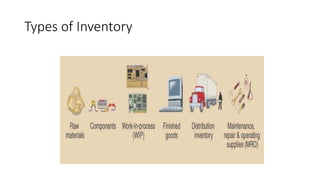
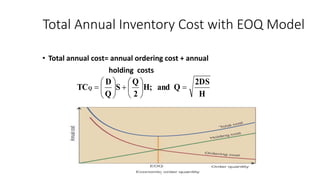
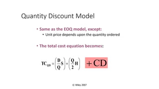
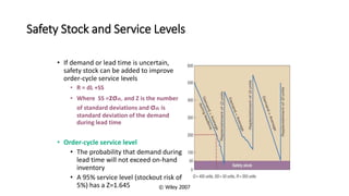
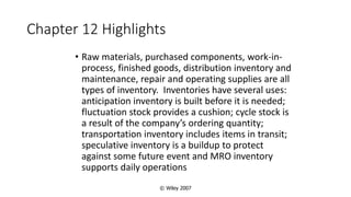
inventory

1. Inventory Models
Hiranya Dissanayake

2. Learning Objectives
• The importance of inventory control systems for organizational
success
• Different types of inventories
• The purpose of holding inventory
• Basic inventory decision problems
• Understanding the EOQ model

3. Inventory
Inventory is any resource that is set aside for
future use

4. The Importance of inventory control systems
• Maintaining and financing inventories represent major cost of doing
business
• The level of inventory is an important decision variable at all stages of
Manufacturing
Financing
Distributing
• Proper inventory control plays a successful operations management
• There are two critical questions
When should we replenish the inventory?
How many units of order at a time?
• It is important to have inventory controls to answer these questions

5. 5
Overview of Inventory Issues
• Proper control of inventory is crucial to the success of
an enterprise.
• Typical inventory problems include:
• Basic inventory – Planned shortage
• Quantity discount – Periodic review
• Production lot size – Single period
• Inventory models are often used to develop an
optimal inventory policy, consisting of:
• An order quantity, denoted Q.
• A reorder point, denoted R.

6. Different types of inventories
• Inventory comes in many shapes and sizes such as
Raw materials – purchased items or extracted materials transformed into
components or products
Components – parts or subassemblies used in final product
Work-in-process – items in process throughout the plant
Finished goods – products sold to customers
Distribution inventory – finished goods in the distribution system
Human resource
Financial and other fixed resource

7. Types of Inventory

8. The purpose of holding inventory
• Satisfaction with fluctuating demand
• Protection against a short supply of materials
• Hedge against price inflation
• Benefits of quantity discounts
• Saving on negotiation costs

9. Basic inventory decision problems
• How much is to be replenished?
• When to be replenished?

10. 10
• Inventory analyses can be thought of as cost-control
techniques.
• Categories of costs in inventory models:
• Holding (carrying costs)
• Order/ Setup costs
• Shortage costs
Type of Costs in Inventory Models

11. 11
• Holding Costs (Carrying costs):
These costs depend on the order
size
• Cost of capital
• Storage space rental cost
• Costs of utilities
• Labor
• Insurance
• Security
• Theft and breakage
• Deterioration or Obsolescence
Ch = Annual holding cost per unit
in inventory
H = Annual holding cost rate
C = Unit cost of an item
Ch = H * C
Type of Costs in Inventory Models

12. 12
• Order/Setup Costs
These costs are independent of the order
size.
• Order costs are incurred when purchasing a
good from a supplier. They include costs such as
• Telephone
• Order checking
• Labor
• Transportation
• Setup costs are incurred when producing goods
for sale to others. They can include costs of
• Cleaning machines
• Calibrating equipment
• Training staff
Type of Costs in Inventory Models
Co = Order cost
or setup cost

13. Shortage Costs
• Costs that occur when demand exceeds the available inventory in
stock.

14. © Wiley 2007
Three Mathematical Models for Determining
Order Quantity
• Economic Order Quantity (EOQ or Q System)
• An optimizing method used for determining order quantity
and reorder points
• Part of continuous review system which tracks on-hand
inventory each time a withdrawal is made
• Economic Production Quantity (EPQ)
• A model that allows for incremental product delivery
• Quantity Discount Model
• Modifies the EOQ process to consider cases where quantity
discounts are available

15. © Wiley 2007
Economic Order Quantity
• EOQ Assumptions:
• Demand is known & constant - no
safety stock is required
• Lead time is known & constant
• No quantity discounts are
available
• Ordering (or setup) costs are
constant
• All demand is satisfied (no
shortages)
• The order quantity arrives in a
single shipment

16. © Wiley 2007
Total Annual Inventory Cost with EOQ Model
• Total annual cost= annual ordering cost + annual
holding costs
H
2DS
Q
and
H;
2
Q
S
Q
D
TCQ 















17. © Wiley 2007
Continuous (Q) Review System Example: A computer company has annual demand of 10,000. They
want to determine EOQ for circuit boards which have an annual holding cost (H) of $6 per unit, and
an ordering cost (S) of $75. They want to calculate TC and the reorder point (R) if the purchasing
lead time is 5 days.
• EOQ (Q)
• Reorder Point (R)
• Total Inventory Cost (TC)
units
500
$6
$75
*
10,000
*
2
H
2DS
Q 


units
200
days
5
*
days
250
10,000
Time
Lead
x
Demand
Daily
R 


$3000
$1500
$1500
$6
2
500
$75
500
10,000
TC 

















18. © Wiley 2007
Economic Production Quantity (EPQ)
• Same assumptions as the EOQ except: inventory arrives in
increments & is drawn down as it arrives

19. © Wiley 2007
EPQ Equations
• Total cost:
• Maximum inventory:
• d=avg. daily demand rate
• p=daily production rate
• Calculating EPQ













 H
2
I
S
Q
D
TC MAX
EPQ










p
d
1
Q
IMAX










p
d
1
H
2DS
EPQ

20. © Wiley 2007
EPQ Problem: HP Ltd. Produces its premium plant food in 50# bags. Demand is 100,000 lbs. per week and they operate 50
wks. each year and HP can produce 250,000 lbs. per week. The setup cost is $200 and the annual holding cost rate is $.55
per bag. Calculate the EPQ. Determine the maximum inventory level. Calculate the total cost of using the EPQ policy.













 H
2
I
S
Q
D
TC MAX
EPQ










p
d
1
H
2DS
EPQ










p
d
1
Q
IMAX

21. © Wiley 2007
EPQ Problem: HP Ltd. Produces its premium plant food in 50# bags. Demand is 100,000 lbs. per week and they operate 50
wks. each year and HP can produce 250,000 lbs. per week. The setup cost is $200 and the annual holding cost rate is $.55
per bag. Calculate the EPQ. Determine the maximum inventory level. Calculate the total cost of using the EPQ policy.










p
d
1
H
2DS
EPQ Bags
EPQ 850
,
77
250000
000
,
100
1
55
.
)
200
)(
000
,
100
)(
50
(
2



















p
d
1
Q
I MAX













 H
2
I
S
Q
D
TC MAX
EPQ
bags
MAX
I 710
,
46
000
,
250
000
,
100
1
850
,
77 










    690
,
25
$
55
.
2
710
,
46
200
850
,
77
000
,
000
,
5















TC

22. © Wiley 2007
Quantity Discount Model
• Same as the EOQ model, except:
• Unit price depends upon the quantity ordered
• The total cost equation becomes:













 H
2
Q
S
Q
D
TCQD CD


23. © Wiley 2007
Quantity Discount Procedure
• Calculate the EOQ at the lowest price
• Determine whether the EOQ is feasible at that price
• Will the vendor sell that quantity at that price?
• If yes, stop – if no, continue
• Check the feasibility of EOQ at the next higher price
• Continue to the next slide ...

24. © Wiley 2007
QD Procedure (continued)
• Continue until you identify a feasible EOQ
• Calculate the total costs (including total item cost) for the feasible
EOQ model
• Calculate the total costs of buying at the minimum quantity required
for each of the cheaper unit prices
• Compare the total cost of each option & choose the lowest cost
alternative
• Any other issues to consider?

25. © Wiley 2007
Quantity Discount Example: Collin’s Sport store is considering going to a different hat supplier. The present
supplier charges $10 each and requires minimum quantities of 490 hats. The annual demand is 12,000 hats,
the ordering cost is $20, and the inventory carrying cost is 20% of the hat cost, a new supplier is offering hats
at $9 in lots of 4000. Who should he buy from?
• EOQ at lowest price $9. Is it feasible?
• Since the EOQ of 516 is not feasible, calculate the total cost (C) for each
price to make the decision
• 4000 hats at $9 each saves $19,320 annually. Space?
hats
516
$1.80
20)
2(12,000)(
EOQ$9 

     
      $101,660
12,000
$9
$1.80
2
4000
$20
4000
12,000
C
$120,980
12,000
$10
$2
2
490
$20
490
12,000
C
$9
$10









26. © Wiley 2007
Safety Stock and Service Levels
• If demand or lead time is uncertain,
safety stock can be added to improve
order-cycle service levels
• R = dL +SS
• Where SS =zσdL, and Z is the number
of standard deviations and σdL is
standard deviation of the demand
during lead time
• Order-cycle service level
• The probability that demand during
lead time will not exceed on-hand
inventory
• A 95% service level (stockout risk of
5%) has a Z=1.645

27. © Wiley 2007
Inventory Management Across the
Organization
• Inventory management policies affect functional areas throughout
• Accounting is concerned of the cost implications of inventory
• Marketing is concerned as stocking decision affect the level of customer
service
• Information Systems is involved to tack and control inventory records

28. © Wiley 2007
Chapter 12 Highlights
• Raw materials, purchased components, work-in-
process, finished goods, distribution inventory and
maintenance, repair and operating supplies are all
types of inventory. Inventories have several uses:
anticipation inventory is built before it is needed;
fluctuation stock provides a cushion; cycle stock is
a result of the company’s ordering quantity;
transportation inventory includes items in transit;
speculative inventory is a buildup to protect
against some future event and MRO inventory
supports daily operations

29. © Wiley 2007
Chapter 12 Highlights
• The objectives of inventory management are to provide the
desired level of customer service, to allow cost-efficient
operations, and to minimize inventory investment.
Customer service can be measured in several ways,
including as a percentage of orders shipped on schedule, a
percentage of line items shipped on schedule, a percentage
of dollar volume shipped on schedule, or idle time due to
material and component shortages. Cots-efficient
operations are achieved by using inventory as buffer stocks
allowing a stable year-round workforce, and spreading the
setup cost over a larger number of Inventory performance
is measured by turns/supply.
• Inventory costs include item cost, holding cost, ordering
cost, and shortage cost.

30. © Wiley 2007
Chapter 12 Highlights (continued)
• Inventory investment is measured in inventory turnover
and/or level of supply. Inventory performance is calculated
as inventory turnover or weeks, days, or hours of supply.
• Relevant inventory costs include items costs, holding costs,
and shortage costs. Holding costs include capital costs,
storage costs, and risk costs. Ordering costs are fixed costs
for placing an order or performing a setup. Shortage costs
included costs related to additional paperwork, additional
shipping expense, and the intangible cost of lost customer
goodwill.

31. © Wiley 2007
Chapter 12 Highlights (continued)
• Lot-for-lot, fixed-order quantity, min-max systems,
order n periods, periodic review systems, EOQ
models, quantity discount models, and single-
period models can be used to determine order
quantities.
• Ordering decisions can be improved by analyzing
total costs of an inventory policy. Total costs
include ordering cost, holding cost, and material
cost

32. © Wiley 2007
Chapter 12 Highlights (continued)
• Practical considerations can cause a company to
not use the optimal order quantity, that is,
minimum order requirements
• Smaller lot sizes give a company flexibility and
shorter response times. The key to reducing order
quantities is to reduce ordering or setup costs.
• Calculating the appropriate safety stock policy
enables companies to satisfy their customer
service objective at minimum costs. The desired
customer service level determines the appropriate
z value.

33. © Wiley 2007
Chapter 12 Highlights (continued)
• Inventory decisions about perishable products can
be made using the single-period inventory model.
The expected payoff is calculated to assist the
quantity decision
• The ABC classification system allows a company to
assign the appropriate level of control and
frequency of review of an item based on its annual
dollar volume
• Cycle counting is a method for maintaining
accurate inventory records. Determining what and
when to count are the major decisions

34. © Wiley 2007
Chapter 12 Highlights (continued)
• Order Q’s can be determined by using L4L, fixed order Q’s, min-max,
order n periods, quantity discounts, and single period systems.
• Ordering decisions can be improved by analyzing TC
• Smaller lot sizes increase flexibility and reduce response time.
• Safety stock can be added to reorder point calculations to meet desired
service level z value.
• Inventory decisions about perishable products can be made by using
the single-period inventory model.
• ABC analysis can be used to assign the appropriate level of control and
review frequency based on the annual dollar volume of each item.
• Cycle counting of pre-specified items is an accepted method for
maintaining inventory records