Download as PDF, PPTX


![Variational Autioencoder
¤ Variational Autoencoder [Kingma+ 13][Rezende+ 14]
¤ 確率分布を多層ニューラルネットワークで表現した⽣成モデル
¤ 単純のため,潜在変数は𝑧のみとする
¤ 最⼤化する下界は
𝐿 𝐱 = 𝐸89 𝐳 𝐱 log
𝑝; 𝐱, 𝐳
𝑞< 𝐳 𝐱
=
1
𝑇
? log
@
ABC
𝑝; 𝐱, 𝐳(𝒕)
𝑞< 𝐳(𝒕) 𝐱
𝑥
𝑧
𝑞(𝑧|𝑥)
近似分布
=エンコーダーと考える
ただし,𝐳(𝒕) = 𝝁 + diag 𝝈 ⨀𝜺, 𝜺~𝑵(𝟎, I)
reparameterization
trick
𝑥~𝑝(𝑥|𝑧)
𝑧~𝑝(𝑧)
デコーダーと考える](https://image.slidesharecdn.com/iclr2016vae-160920054645/85/Iclr2016-vae-8-320.jpg)
![VAEのモデル化
¤ ニューラルネットワークによってモデル化する
・・・
・・・
・・・ ・・・
・・・
・・・
・・・
推論モデル
sampling
z(l)
= µ + σ ⊙ ϵ(l)
, ϵ(l)
∼ N(0, I).
ost significant difference from the estimator of VAE’s lower bound (Eq. (3)) is that there are
gative reconstruction terms in Eq. (8). These terms are correspondent to each modality. Same
, we call qφ(z|x, w) as encoder and both pθx (x|z(l)
) and pθw (w|z(l)
) as decoder.
parameterize encoder and decoder distribution as deep neural networks. Figs.2 draws the
which is same as Fig. 1 but represented by deep neural networks.
ering the encoder qφ(z|x, w) as a Gaussian distribution, we can estimate mean and variance
istribution by neural networks as follows:
y(x) = MLPφx (x)
y(w) = MLPφw (w)
µφ = Linear(y(x), y(w))
log σ2
φ = Tanh(Linear(y(x), y(w)), (9)
MLPφx and MLPφw mean deep neural networks corresponding each modality. Moreover,
r and Tanh mean a linear layer and a tanh layer. Linear(a, b) means that this network has
e input layers, which are corresponding to a and b.
e each modality has different feature representation, we should make different networks for
coder, pθx (x|z) and pθw (w|z). The type of distribution and the network architecture depend
epresentation of each modality, e.g., Gaussian distribution when the representation of modal-
ntinuous, Bernoulli distribution when binary value, 0 or 1. In case that pθw (w|z) is Bernoulli
tion B(w|µθw
), the parameter of Bernoulli distribution µθw
can estimate as follows:
y(z) = MLPθw (z)
µθ = Linear(y(z)) (10)
that the decoder is Gaussian distribution, you can estimate the parameter of this distribution
where z(l)
= µ + σ ⊙ ϵ(l)
, ϵ(l)
∼ N(0, I).
The most significant difference from the estimator of VAE’s lower bound (Eq. (3)) is that there are
two negative reconstruction terms in Eq. (8). These terms are correspondent to each modality. Same
as VAE, we call qφ(z|x, w) as encoder and both pθx (x|z(l)
) and pθw (w|z(l)
) as decoder.
We can parameterize encoder and decoder distribution as deep neural networks. Figs.2 draws the
model which is same as Fig. 1 but represented by deep neural networks.
Considering the encoder qφ(z|x, w) as a Gaussian distribution, we can estimate mean and variance
of the distribution by neural networks as follows:
y(x) = MLPφx (x)
y(w) = MLPφw (w)
µφ = Linear(y(x), y(w))
log σ2
φ = Tanh(Linear(y(x), y(w)), (9)
where MLPφx and MLPφw mean deep neural networks corresponding each modality. Moreover,
Linear and Tanh mean a linear layer and a tanh layer. Linear(a, b) means that this network has
multiple input layers, which are corresponding to a and b.
Because each modality has different feature representation, we should make different networks for
each decoder, pθx (x|z) and pθw (w|z). The type of distribution and the network architecture depend
on the representation of each modality, e.g., Gaussian distribution when the representation of modal-
ity is continuous, Bernoulli distribution when binary value, 0 or 1. In case that pθw (w|z) is Bernoulli
distribution B(w|µθw
), the parameter of Bernoulli distribution µθw
can estimate as follows:
y(z) = MLPθw (z)
µθ = Linear(y(z)) (10)
In case that the decoder is Gaussian distribution, you can estimate the parameter of this distribution
in the same way as Eq. (9), except that the input of the Linear network is single.
The main advantage of this model is following:
Figure 2: The network architecture of MVAE. This represents the sam
Hense,
L(x, w) = −DKL(qφ(z|x, w)||p(z))
+Eqφ(z|x,w)[log pθx (x|z)] + Eqφ(z|x,w)[log p
By SGBM algorithm, the estimator of the lower bound is as follows:
ˆL(x, w) = −DKL(qφ(z|x, w)||p(z))
+
1
L
L
l=1
log pθx (x|z(l)
) + log pθw (w|z(
where z(l)
= µ + σ ⊙ ϵ(l)
, ϵ(l)
∼ N(0, I).
The most significant difference from the estimator of VAE’s lower bound (E
two negative reconstruction terms in Eq. (8). These terms are correspondent
as VAE, we call qφ(z|x, w) as encoder and both pθx (x|z(l)
) and pθw (w|z(l)
We can parameterize encoder and decoder distribution as deep neural netw
model which is same as Fig. 1 but represented by deep neural networks.
$ #% $&
rk architecture of MVAE. This represents the same model as Fig.1.
= −DKL(qφ(z|x, w)||p(z))
+Eqφ(z|x,w)[log pθx (x|z)] + Eqφ(z|x,w)[log pθw (w|z)] (7)
estimator of the lower bound is as follows:
w) = −DKL(qφ(z|x, w)||p(z))
+
1
L
L
l=1
log pθx (x|z(l)
) + log pθw (w|z(l)
), (8)
, ϵ(l)
∼ N(0, I).
ence from the estimator of VAE’s lower bound (Eq. (3)) is that there are
・・・ ・・・
settings and found that their proposed model can extract better representations than sing
settings.
Srivastava & Salakhutdinov (2012) used deep restricted Boltzmann machines (RBM), w
earliest deep generative model, to multimodal learning settings. The same as one by usin
they jointed latent variables in multiple networks and tried to extract high-level feature
timodal features: images and texts. In their experiment, they showed that their model ou
Ngiam et al. (2011). It suggests that deep generative models may extract better represen
discriminative ones.
2.2 VARIATIONAL AUTOENCODERS
Variational autoencoders (VAE) (Welling, 2014; Rezende et al., 2014) are recent propose
erative models.
Given observation variables x and corresponding latent variables z, we consider their
processes as follow:
z ∼ p(z); x ∼ pθ(x|z), ˆx ˆw
where θ means the model parameter of p.
In varaitional inference, we consider qφ(z|x), where φ is the model parameter of q, in
proximate the posterior distribution pθ(z|x). The goal of this problem is that maximize t
𝑞(𝑧|𝑥)
𝑥~𝑝(𝑥|𝑧)
𝑧~𝑝(𝑧)
⽣成モデル](https://image.slidesharecdn.com/iclr2016vae-160920054645/85/Iclr2016-vae-9-320.jpg)
![Importance Weighted AE
¤ Importance Weighted Autoencoders [Bruda+ 15; ICLR 2016]
¤ 次のような新たな下界を提案
¤ サンプル数kによる重要度重み推定量
𝐿# 𝑥 = 𝐸RS,…,RU~89 𝑧 𝑥 log
1
𝑘
?
𝑝; 𝐱, 𝐳(𝐤)
𝑞< 𝐳(𝐤)
𝐱
X
#BC
¤ この下界は,次の関係が証明されている
log 𝑝 𝑥 ≥ 𝐿#ZC 𝑥 ≥ 𝐿# 𝑥 ≥ 𝐿C 𝑥 = 𝐿 𝑥
¤ サンプル数を増やすだけで,制約が緩和され,真の下界に近づく.](https://image.slidesharecdn.com/iclr2016vae-160920054645/85/Iclr2016-vae-11-320.jpg)

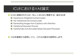
![VAEによる半教師あり学習
¤ Semi-Supervised Learning with Deep Generative Models
[Kingma+ 2014 ; NIPS 2014]
¤ 条件付きVAE(CVAE)による半教師あり学習
¤ 条件付きVAEの下界は 𝐿 𝐱|𝒚 = 𝐸89 𝐳 𝐱, 𝐲 log
]^ 𝐱,𝐳|𝐲
89 𝐳 𝐱, 𝐲
¤ よって,下界は
𝐿 𝐱 + 𝐿 𝐱|𝐲 + 𝛼𝔼[−log𝑞< 𝐲 𝐱 ]
¤ 最後の項はラベル予測するモデル
𝑧
𝑥
𝑦
ラベル](https://image.slidesharecdn.com/iclr2016vae-160920054645/85/Iclr2016-vae-14-320.jpg)
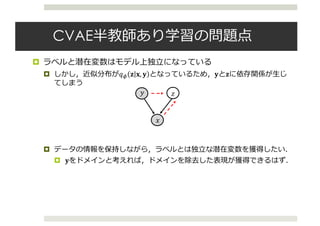
![Variational Fair Autoencoder
¤ The Variational Fair Autoencoder [Louizos+ 15; ICLR 2016]
¤ 𝑥と𝑠(sensitive変数.前ページでいうラベル)を独⽴にするために,次の
maximum mean discrepancy(MMD)を⼩さくするようにする.
¤ s=0とs=1のときの潜在変数の差がなくなるようにする.
¤ これをVAEの下界に追加する.
¤ MMDは通常カーネルの計算に持っていく.
¤ しかし,SGDで⾼次元のグラム⾏列を計算するのは⼤変なので,写像
を次の形で求める
(7)
Asymptotically, for a universal kernel such as the Gaussian kernel k(x, x0
) = e kx x0
k2
,
`MMD(X, X0
) is 0 if and only if P0 = P1. Equivalently, minimizing MMD can be viewed as
matching all of the moments of P0 and P1. Therefore, we can use it as an extra “regularizer” and
force the model to try to match the moments between the marginal posterior distributions of our
latent variables, i.e., q (z1|s = 0) and q (z1|s = 1) (in the case of binary nuisance information
s1
). By adding the MMD penalty into the lower bound of our aforementioned VAE architecture we
obtain our proposed model, the “Variational Fair Autoencoder” (VFAE):
FVFAE( , ✓; xn, xm, sn, sm, yn) = FVAE( , ✓; xn, xm, sn, sm, yn) `MMD(Z1s=0, Z1s=1) (8)
where:
`MMD(Z1s=0, Z1s=1) = k E˜p(x|s=0)[Eq(z1|x,s=0)[ (z1)]] E˜p(x|s=1)[Eq(z1|x,s=1)[ (z1)]]k2
(9)
2.4 FAST MMD VIA RANDOM FOURIER FEATURES
A naive implementation of MMD in minibatch stochastic gradient descent would require computing
the M ⇥M Gram matrix for each minibatch during training, where M is the minibatch size. Instead,
we can use random kitchen sinks (Rahimi & Recht, 2009) to compute a feature expansion such that
computing the estimator (6) approximates the full MMD (7). To compute this, we draw a random
K ⇥ D matrix W, where K is the dimensionality of x, D is the number of random features and
each entry of W is drawn from a standard isotropic Gaussian. The feature expansion is then given
as:
W(x) =
r
2
D
cos
✓r
2
xW + b
◆
. (10)
where b is a D-dimensional uniform random vector with entries in [0, 2⇡]. Zhao & Meng (2015)
have successfully applied the idea of using random kitchen sinks to approximate MMD. This esti-
mator is fairly accurate, and is typically much faster than the full MMD penalty. We use D = 500
et al., 2006):
`MMD(X, X0
) =
1
N2
0
N0X
n=1
N0X
m=1
k(xn, xm) +
1
N2
1
N1X
n=1
N1X
m=1
k(x0
n, x0
m)
2
N0N1
N0X
n=1
N1X
m=1
k(xn, x0
m).
(7)
Asymptotically, for a universal kernel such as the Gaussian kernel k(x, x0
) = e kx x0
k2
,
`MMD(X, X0
) is 0 if and only if P0 = P1. Equivalently, minimizing MMD can be viewed as
matching all of the moments of P0 and P1. Therefore, we can use it as an extra “regularizer” and
force the model to try to match the moments between the marginal posterior distributions of our
latent variables, i.e., q (z1|s = 0) and q (z1|s = 1) (in the case of binary nuisance information
s1
). By adding the MMD penalty into the lower bound of our aforementioned VAE architecture we
obtain our proposed model, the “Variational Fair Autoencoder” (VFAE):
FVFAE( , ✓; xn, xm, sn, sm, yn) = FVAE( , ✓; xn, xm, sn, sm, yn) `MMD(Z1s=0, Z1s=1) (8)
where:
`MMD(Z1s=0, Z1s=1) = k E˜p(x|s=0)[Eq(z1|x,s=0)[ (z1)]] E˜p(x|s=1)[Eq(z1|x,s=1)[ (z1)]]k2
(9)
2.4 FAST MMD VIA RANDOM FOURIER FEATURES
A naive implementation of MMD in minibatch stochastic gradient descent would require computing
the M ⇥M Gram matrix for each minibatch during training, where M is the minibatch size. Instead,
we can use random kitchen sinks (Rahimi & Recht, 2009) to compute a feature expansion such that
computing the estimator (6) approximates the full MMD (7). To compute this, we draw a random
K ⇥ D matrix W, where K is the dimensionality of x, D is the number of random features and
each entry of W is drawn from a standard isotropic Gaussian. The feature expansion is then given
as:
W(x) =
r
2
D
cos
✓r
2
xW + b
◆
. (10)
where b is a D-dimensional uniform random vector with entries in [0, 2⇡]. Zhao & Meng (2015)
have successfully applied the idea of using random kitchen sinks to approximate MMD. This esti-
mator is fairly accurate, and is typically much faster than the full MMD penalty. We use D = 500
in our experiments.](https://image.slidesharecdn.com/iclr2016vae-160920054645/85/Iclr2016-vae-16-320.jpg)
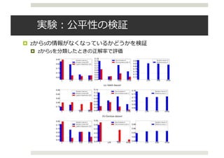
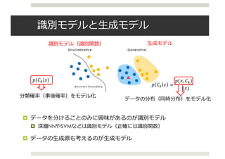
![実験:ドメイン適応の検証
¤ 異なるドメイン間でのドメイン適応
¤ 半教師あり学習で実験(⽬標ドメインのラベルがない).
¤ the Amazon reviews dataset
¤ 𝑦はセンチメント(positiveかnegative)
¤ 結果:
¤ 12のうち9が既存研究([Ganin+ 15])を上回った
Under review as a conference paper at ICLR 2016
2 LEARNING INVARIANT REPRESENTATIONS
x
zs
N
Figure 1: Unsupervised model
x
z1s
z2
y
N
Figure 2: Semi-supervised model
2.1 UNSUPERVISED MODEL
Factoring out undesired variations from the data can be easily formulated as a general probabili
model which admits two distinct (independent) “sources”; an observed variable s, which denotes
variations that we want to remove, and a continuous latent variable z which models all the remain
information. This generative process can be formally defined as:
z ⇠ p(z); x ⇠ p✓(x|z, s)
where p✓(x|z, s) is an appropriate probability distribution for the data we are modelling. With
formulation we explicitly encode a notion of ‘invariance’ in our model, since the latent repres
Under review as a conference paper at ICLR 2016
is concerned, we compared against a recent neural network based state of the art method for domain
adaptation, Domain Adversarial Neural Network (DANN) (Ganin et al., 2015). As we can observe
in table 1, our accuracy on the labels y is higher on 9 out of the 12 domain adaptation tasks whereas
on the remaining 3 it is quite similar to the DANN architecture.
Table 1: Results on the Amazon reviews dataset. The DANN column is taken directly from Ganin
et al. (2015) (the column that uses the original representation as input).
Source - Target
S Y
RF LR VFAE DANN
books - dvd 0.535 0.564 0.799 0.784
books - electronics 0.541 0.562 0.792 0.733
books - kitchen 0.537 0.583 0.816 0.779
dvd - books 0.537 0.563 0.755 0.723
dvd - electronics 0.538 0.566 0.786 0.754
dvd - kitchen 0.543 0.589 0.822 0.783
electronics - books 0.562 0.590 0.727 0.713
electronics - dvd 0.556 0.586 0.765 0.738
electronics - kitchen 0.536 0.570 0.850 0.854
kitchen - books 0.560 0.593 0.720 0.709
kitchen - dvd 0.561 0.599 0.733 0.740
kitchen - electronics 0.533 0.565 0.838 0.843](https://image.slidesharecdn.com/iclr2016vae-160920054645/85/Iclr2016-vae-18-320.jpg)
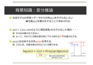
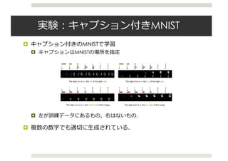
![CVAEの活⽤
¤ 条件付きVAEは,ラベル等に条件づけられた画像を⽣成できる
¤ 学習サンプルに存在していないデータも⽣成可能
¤ 数字ラベルで条件付け[Kingma+ 2014 ; NIPS 2014]
(a) Handwriting styles for MNIST obtained by fixing the class label and varying the 2D latent variable z
(b) MNIST analogies (c) SVHN analogies
Figure 1: (a) Visualisation of handwriting styles learned by the model with 2D z-space. (b,c)
Analogical reasoning with generative semi-supervised models using a high-dimensional z-space.
The leftmost columns show images from the test set. The other columns show analogical fantasies
of x by the generative model, where the latent variable z of each row is set to the value inferred from](https://image.slidesharecdn.com/iclr2016vae-160920054645/85/Iclr2016-vae-19-320.jpg)
![Conditional alignDRAW
¤ Generating Images from Captions with Attention [Mansimov+
16 ; ICLR 2016]
¤ DRAWにbidirectional RNNで条件づけたモデル
¤ DRAW [Gregor+ 14]
¤ VAEの枠組みでRNNを使えるようにしたもの.
¤ 各時間ステップで画像を上書きしていく
¤ 前のステップとの差分をみることで注意(attention)をモデル化
Recurrent Neural Network For Image Generation
onstructs scenes
s emitted by the
encoder.
s step by step is
the scene while
e past few years
captured by a se-
, than by a sin-
chelle & Hinton,
; Ranzato, 2014;
et al., 2014; Ser-
ed by sequential
read
x
zt zt+1
P(x|z1:T )write
encoder
RNN
sample
decoder
RNN
read
x
write
encoder
RNN
sample
decoder
RNN
ct 1 ct cT
henc
t 1
hdec
t 1
Q(zt|x, z1:t 1) Q(zt+1|x, z1:t)
. . .
decoding
(generative model)
encoding
(inference)
encoder
FNN
sample
decoder
FNN
z
P(x|z)
Figure 2. Left: Conventional Variational Auto-Encoder. Dur-
DRAW: A Recurrent Neural Network For Image Generati
Time
Figure 7. MNIST generation sequences for DRAW without at-
tention. Notice how the network first generates a very blurry im-](https://image.slidesharecdn.com/iclr2016vae-160920054645/85/Iclr2016-vae-20-320.jpg)
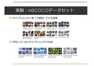
![Conditional alignDRAW
¤ Conditional alignDRAWの全体像
¤ DRAWにbidirectional RNNで条件づけたモデル
¤ Bidirectional RNNの出⼒を重み付け和したもので条件付ける.
Published as a conference paper at ICLR 2016
Figure 2: AlignDRAW model for generating images by learning an alignment between the input captions and
generating canvas. The caption is encoded using the Bidirectional RNN (left). The generative RNN takes a
latent sequence z1:T sampled from the prior along with the dynamic caption representation s1:T to generate
the canvas matrix cT , which is then used to generate the final image x (right). The inference RNN is used to
compute approximate posterior Q over the latent sequence.
3.2 IMAGE MODEL: THE CONDITIONAL DRAW NETWORK
To generate an image x conditioned on the caption information y, we extended the DRAW net-
work (Gregor et al., 2015) to include caption representation hlang
at each step, as shown in Fig. 2.
The conditional DRAW network is a stochastic recurrent neural network that consists of a sequence
of latent variables Zt 2 RD
, t = 1, .., T, where the output is accumulated over all T time-steps. For
simplicity in notation, the images x 2 Rh⇥w
are assumed to have size h-by-w and only one color
𝑦
𝑥
𝑧
3.3 LEARNING
The model is trained to maximize a variational lower bound L on the marginal likelihood of the
correct image x given the input caption y:
L =
X
Z
Q(Z | x, y) log P(x | y, Z) DKL (Q(Z | x, y) k P(Z | y)) log P(x | y). (9)
Similar to the DRAW model, the inference recurrent network produces an approximate posterior
Q(Z1:T | x, y) via a read operator, which reads a patch from an input image x using two arrays of
1D Gaussian filters (inverse of write from section 3.2) at each time-step t. Specifically,
ˆxt = x (ct 1), (10)
rt = read(xt, ˆxt, hgen
t 1), (11)
hinfer
t = LSTM infer
(hinfer
t 1 , [rt, hgen
t 1]), (12)
Q(Zt|x, y, Z1:t 1) = N
⇣
µ(hinfer
t ), (hinfer
t )
⌘
, (13)
where ˆx is the error image and hinfer
0 is initialized to the learned bias b. Note that the inference
LSTM infer
takes as its input both the output of the read operator rt 2 Rp⇥p
, which depends on
the original input image x, and the previous state of the generative decoder hgen
t 1, which depends
on the latent sample history z1:t 1 and dynamic sentence representation st 1 (see Eq. 3). Hence,
the approximate posterior Q will depend on the input image x, the corresponding caption y, and the
latent history Z1:t 1, except for the first step Q(Z1|x), which depends only on x.
The terms in the variational lower bound Eq. 9 can be rearranged using the law of total expectation.
Therefore, the variational bound L is calculated as follows:
L =EQ(Z1:T | y,x)
"
log p(x | y, Z1:T )
TX
t=2
DKL (Q(Zt | Z1:t 1, y, x) k P(Zt | Z1:t 1, y))
#
DKL (Q(Z1 | x) k P(Z1)) . (14)
1
We also experimented with a conditional Gaussian observation model, but it worked worse compared to
the Bernoulli model.](https://image.slidesharecdn.com/iclr2016vae-160920054645/85/Iclr2016-vae-21-320.jpg)

![ガウス過程
¤ ガウス過程とは・・・
¤ 関数の確率分布
¤ D次元の⼊⼒ベクトルのデータセット に対する関数の出⼒
ベクトル の同時分布が常にガウス分布
¤ 平均ベクトルは ,共分散⾏列は で完全に記
述される
an Processes
ew the predictive equations and marginal likelihood for Gaussian processes
e associated computational requirements, following the notational conven-
n et al. (2015). See, for example, Rasmussen and Williams (2006) for a
discussion of GPs.
ataset D of n input (predictor) vectors X = {x1, . . . , xn}, each of dimension
x an n ⇥ 1 vector of targets y = (y(x1), . . . , y(xn))>. If f(x) ⇠ GP(µ, k ),
tion of function values f has a joint Gaussian distribution,
f = f(X) = [f(x1), . . . , f(xn)]>
⇠ N(µ, KX,X) , (1)
ector, µi = µ(xi), and covariance matrix, (KX,X)ij = k (xi, xj), determined
function and covariance kernel of the Gaussian process. The kernel, k , is
y . Assuming additive Gaussian noise, y(x)|f(x) ⇠ N(y(x); f(x), 2), the
ibution of the GP evaluated at the n⇤ test points indexed by X⇤, is given by
f⇤|X⇤,X, y, , 2
⇠ N(E[f⇤], cov(f⇤)) , (2)
E[f⇤] = µX⇤
+ KX⇤,X[KX,X + 2
I] 1
y ,
cov(f⇤) = KX⇤,X⇤ KX⇤,X[KX,X + 2
I] 1
KX,X⇤ .
mple, is an n⇤ ⇥ n matrix of covariances between the GP evaluated at X⇤
3 Gaussian Processes
We briefly review the predictive equations and marginal likelihood for Gaussian processes
(GPs), and the associated computational requirements, following the notational conven-
tions in Wilson et al. (2015). See, for example, Rasmussen and Williams (2006) for a
comprehensive discussion of GPs.
We assume a dataset D of n input (predictor) vectors X = {x1, . . . , xn}, each of dimension
D, which index an n ⇥ 1 vector of targets y = (y(x1), . . . , y(xn))>. If f(x) ⇠ GP(µ, k ),
then any collection of function values f has a joint Gaussian distribution,
f = f(X) = [f(x1), . . . , f(xn)]>
⇠ N(µ, KX,X) , (1)
with a mean vector, µi = µ(xi), and covariance matrix, (KX,X)ij = k (xi, xj), determined
from the mean function and covariance kernel of the Gaussian process. The kernel, k , is
parametrized by . Assuming additive Gaussian noise, y(x)|f(x) ⇠ N(y(x); f(x), 2), the
predictive distribution of the GP evaluated at the n⇤ test points indexed by X⇤, is given by
f⇤|X⇤,X, y, , 2
⇠ N(E[f⇤], cov(f⇤)) , (2)
E[f⇤] = µX⇤
+ KX⇤,X[KX,X + 2
I] 1
y ,
cov(f⇤) = KX⇤,X⇤ KX⇤,X[KX,X + 2
I] 1
KX,X⇤ .
KX⇤,X, for example, is an n⇤ ⇥ n matrix of covariances between the GP evaluated at X⇤
We briefly review the predictive equations and marginal likelihood for Gaussian proc
(GPs), and the associated computational requirements, following the notational con
tions in Wilson et al. (2015). See, for example, Rasmussen and Williams (2006) f
comprehensive discussion of GPs.
We assume a dataset D of n input (predictor) vectors X = {x1, . . . , xn}, each of dimen
D, which index an n ⇥ 1 vector of targets y = (y(x1), . . . , y(xn))>. If f(x) ⇠ GP(µ,
then any collection of function values f has a joint Gaussian distribution,
f = f(X) = [f(x1), . . . , f(xn)]>
⇠ N(µ, KX,X) ,
with a mean vector, µi = µ(xi), and covariance matrix, (KX,X)ij = k (xi, xj), determ
from the mean function and covariance kernel of the Gaussian process. The kernel, k
parametrized by . Assuming additive Gaussian noise, y(x)|f(x) ⇠ N(y(x); f(x), 2)
predictive distribution of the GP evaluated at the n⇤ test points indexed by X⇤, is give
f⇤|X⇤,X, y, , 2
⇠ N(E[f⇤], cov(f⇤)) ,
E[f⇤] = µX⇤
+ KX⇤,X[KX,X + 2
I] 1
y ,
cov(f⇤) = KX⇤,X⇤ KX⇤,X[KX,X + 2
I] 1
KX,X⇤ .
and Nickisch, 2015) and extensions in Wilson et al. (2015) for e ciently representing kernel
functions, to produce scalable deep kernels.
3 Gaussian Processes
We briefly review the predictive equations and marginal likelihood for Gaussian processes
(GPs), and the associated computational requirements, following the notational conven-
tions in Wilson et al. (2015). See, for example, Rasmussen and Williams (2006) for a
comprehensive discussion of GPs.
We assume a dataset D of n input (predictor) vectors X = {x1, . . . , xn}, each of dimension
D, which index an n ⇥ 1 vector of targets y = (y(x1), . . . , y(xn))>. If f(x) ⇠ GP(µ, k ),
then any collection of function values f has a joint Gaussian distribution,
f = f(X) = [f(x1), . . . , f(xn)]>
⇠ N(µ, KX,X) , (1)
with a mean vector, µi = µ(xi), and covariance matrix, (KX,X)ij = k (xi, xj), determined
from the mean function and covariance kernel of the Gaussian process. The kernel, k , is
parametrized by . Assuming additive Gaussian noise, y(x)|f(x) ⇠ N(y(x); f(x), 2), the
predictive distribution of the GP evaluated at the n⇤ test points indexed by X⇤, is given by
f⇤|X⇤,X, y, , 2
⇠ N(E[f⇤], cov(f⇤)) , (2)
E[f⇤] = µX⇤
+ KX⇤,X[KX,X + 2
I] 1
y ,
cov(f⇤) = KX⇤,X⇤ KX⇤,X[KX,X + 2
I] 1
KX,X⇤ .
KX⇤,X, for example, is an n⇤ ⇥ n matrix of covariances between the GP evaluated at X⇤
and X. µX⇤
is the n⇤ ⇥ 1 mean vector, and KX,X is the n ⇥ n covariance matrix evaluated
show that the proposed model outperforms state of the art stand-alone deep learning archi-
tectures and Gaussian processes with advanced kernel learning procedures on a wide range
of datasets, demonstrating its practical significance. We achieve scalability while retaining
non-parametric model structure by leveraging the very recent KISS-GP approach (Wilson
and Nickisch, 2015) and extensions in Wilson et al. (2015) for e ciently representing kernel
functions, to produce scalable deep kernels.
3 Gaussian Processes
We briefly review the predictive equations and marginal likelihood for Gaussian processes
(GPs), and the associated computational requirements, following the notational conven-
tions in Wilson et al. (2015). See, for example, Rasmussen and Williams (2006) for a
comprehensive discussion of GPs.
We assume a dataset D of n input (predictor) vectors X = {x1, . . . , xn}, each of dimension
D, which index an n ⇥ 1 vector of targets y = (y(x1), . . . , y(xn))>. If f(x) ⇠ GP(µ, k ),
then any collection of function values f has a joint Gaussian distribution,
f = f(X) = [f(x1), . . . , f(xn)]>
⇠ N(µ, KX,X) , (1)
with a mean vector, µi = µ(xi), and covariance matrix, (KX,X)ij = k (xi, xj), determined
from the mean function and covariance kernel of the Gaussian process. The kernel, k , is
parametrized by . Assuming additive Gaussian noise, y(x)|f(x) ⇠ N(y(x); f(x), 2), the
predictive distribution of the GP evaluated at the n⇤ test points indexed by X⇤, is given by
f⇤|X⇤,X, y, , 2
⇠ N(E[f⇤], cov(f⇤)) , (2)
E[f⇤] = µX⇤
+ KX⇤,X[KX,X + 2
I] 1
y ,
cov(f⇤) = KX⇤,X⇤ KX⇤,X[KX,X + 2
I] 1
KX,X⇤ .
KX⇤,X, for example, is an n⇤ ⇥ n matrix of covariances between the GP evaluated at X⇤
and X. µX⇤
is the n⇤ ⇥ 1 mean vector, and KX,X is the n ⇥ n covariance matrix evaluated
at training inputs X. All covariance (kernel) matrices implicitly depend on the kernel
hyperparameters .
15.2. GPs for regression 517
−5 0 5
−2
−1.5
−1
−0.5
0
0.5
1
1.5
2
(a)
−5 0 5
−2
−1.5
−1
−0.5
0
0.5
1
1.5
2
2.5
(b)
Figure 15.2 Left: some functions sampled from a GP prior with SE kernel. Right: some samples from a GP
posterior, after conditioning on 5 noise-free observations. The shaded area represents E [f(x)]±2std(f(x).
ns and marginal likelihood for Gaussian processes
al requirements, following the notational conven-
example, Rasmussen and Williams (2006) for a
ctor) vectors X = {x1, . . . , xn}, each of dimension
ets y = (y(x1), . . . , y(xn))>. If f(x) ⇠ GP(µ, k ),
has a joint Gaussian distribution,
. . . , f(xn)]>
⇠ N(µ, KX,X) , (1)
ariance matrix, (KX,X)ij = k (xi, xj), determined
kernel of the Gaussian process. The kernel, k , is
Gaussian noise, y(x)|f(x) ⇠ N(y(x); f(x), 2), the
ed at the n⇤ test points indexed by X⇤, is given by
N(E[f⇤], cov(f⇤)) , (2)
X⇤,X[KX,X + 2
I] 1
y ,
KX⇤,X[KX,X + 2
I] 1
KX,X⇤ .
x of covariances between the GP evaluated at X⇤
nd KX,X is the n ⇥ n covariance matrix evaluated](https://image.slidesharecdn.com/iclr2016vae-160920054645/85/Iclr2016-vae-25-320.jpg)
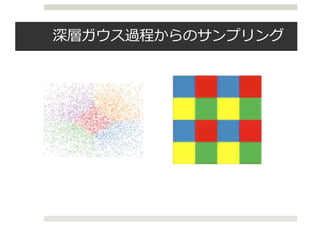
![深層ガウス過程
¤ より複雑なサンプルを表現するため,process compositionによって
多層化する[Lawrence & Moore, 07]
➡ 深層ガウス過程(deep GP)
¤ 以下のように,多層グラフィカルモデルを考える
¤ ここでは𝑌がデータ,𝑋が潜在変数.
Published as a conference paper at ICLR 2016
X3 X2
f1 ⇠ GP
X1
f2 ⇠ GP
Y
f3 ⇠ GP
Figure 1: A deep Gaussian process with two hidden layers.
2 DEEP GAUSSIAN PROCESSES
Gaussian processes provide flexible, non-parametric, probabilistic approaches to function estima-
tion. However, their tractability comes at a price: they can only represent a restricted class of
functions. Indeed, even though sophisticated definitions and combinations of covariance functions
can lead to powerful models (Durrande et al., 2011; G¨onen & Alpaydin, 2011; Hensman et al.,
2013; Duvenaud et al., 2013; Wilson & Adams, 2013), the assumption about joint normal distribu-
tion of instantiations of the latent function remains; this limits the applicability of the models. One
line of recent research to address this limitation focused on function composition (Snelson et al.,
2004; Calandra et al., 2014). Inspired by deep neural networks, a deep Gaussian process instead
employs process composition (Lawrence & Moore, 2007; Damianou et al., 2011; L´azaro-Gredilla,
2012; Damianou & Lawrence, 2013; Hensman & Lawrence, 2014).
A deep GP is a deep directed graphical model that consists of multiple layers of latent variables
and employs Gaussian processes to govern the mapping between consecutive layers (Lawrence &
Moore, 2007; Damianou, 2015). Observed outputs are placed in the down-most layer and observed
inputs (if any) are placed in the upper-most layer, as illustrated in Figure 1. More formally, consider
a set of data Y 2 RN⇥D
with N datapoints and D dimensions. A deep GP then defines L layers of
latent variables, {Xl}L
l=1, Xl 2 RN⇥Ql
through the following nested noise model definition:
Y = f1(X1) + ✏1, ✏1 ⇠ N(0, 2
1I) (1)
Xl 1 = fl(Xl) + ✏l, ✏l ⇠ N(0, 2
l I), l = 2 . . . L (2)
where the functions fl are drawn from Gaussian processes with covariance functions kl, i.e. fl(x) ⇠
GP(0, kl(x, x0
)). In the unsupervised case, the top hidden layer is assigned a unit Gaussian as
a fairly uninformative prior which also provides soft regularization, i.e. XL ⇠ N(0, I). In the
supervised learning scenario, the inputs of the top hidden layer is observed and govern its hidden
outputs.
The expressive power of a deep GP is significantly greater than that of a standard GP, because the
successive warping of latent variables through the hierarchy allows for modeling non-stationarities
and sophisticated, non-parametric functional “features” (see Figure 2). Similarly to how a GP is
EEP GAUSSIAN PROCESSES
n processes provide flexible, non-parametric, probabilistic approaches to function estima-
However, their tractability comes at a price: they can only represent a restricted class of
ns. Indeed, even though sophisticated definitions and combinations of covariance functions
d to powerful models (Durrande et al., 2011; G¨onen & Alpaydin, 2011; Hensman et al.,
Duvenaud et al., 2013; Wilson & Adams, 2013), the assumption about joint normal distribu-
nstantiations of the latent function remains; this limits the applicability of the models. One
recent research to address this limitation focused on function composition (Snelson et al.,
Calandra et al., 2014). Inspired by deep neural networks, a deep Gaussian process instead
s process composition (Lawrence & Moore, 2007; Damianou et al., 2011; L´azaro-Gredilla,
Damianou & Lawrence, 2013; Hensman & Lawrence, 2014).
GP is a deep directed graphical model that consists of multiple layers of latent variables
ploys Gaussian processes to govern the mapping between consecutive layers (Lawrence &
2007; Damianou, 2015). Observed outputs are placed in the down-most layer and observed
if any) are placed in the upper-most layer, as illustrated in Figure 1. More formally, consider
data Y 2 RN⇥D
with N datapoints and D dimensions. A deep GP then defines L layers of
ariables, {Xl}L
l=1, Xl 2 RN⇥Ql
through the following nested noise model definition:
Y = f1(X1) + ✏1, ✏1 ⇠ N(0, 2
1I) (1)
Xl 1 = fl(Xl) + ✏l, ✏l ⇠ N(0, 2
l I), l = 2 . . . L (2)
he functions fl are drawn from Gaussian processes with covariance functions kl, i.e. fl(x) ⇠
kl(x, x0
)). In the unsupervised case, the top hidden layer is assigned a unit Gaussian as
uninformative prior which also provides soft regularization, i.e. XL ⇠ N(0, I). In the
sed learning scenario, the inputs of the top hidden layer is observed and govern its hidden
pressive power of a deep GP is significantly greater than that of a standard GP, because the
ive warping of latent variables through the hierarchy allows for modeling non-stationarities
histicated, non-parametric functional “features” (see Figure 2). Similarly to how a GP is
t of an infinitely wide neural network, a deep GP is the limit where the parametric function
ition of a deep neural network turns into a process composition. Specifically, a deep neural
2 DEEP GAUSSIAN PROCESSES
Gaussian processes provide flexible, non-parame
tion. However, their tractability comes at a pric
functions. Indeed, even though sophisticated defi
can lead to powerful models (Durrande et al., 2
2013; Duvenaud et al., 2013; Wilson & Adams, 2
tion of instantiations of the latent function remain
line of recent research to address this limitation
2004; Calandra et al., 2014). Inspired by deep n
employs process composition (Lawrence & Moor
2012; Damianou & Lawrence, 2013; Hensman &
A deep GP is a deep directed graphical model th
and employs Gaussian processes to govern the m
Moore, 2007; Damianou, 2015). Observed output
inputs (if any) are placed in the upper-most layer, a
a set of data Y 2 RN⇥D
with N datapoints and D
latent variables, {Xl}L
l=1, Xl 2 RN⇥Ql
through th
Y = f1(X1) + ✏1, ✏1
Xl 1 = fl(Xl) + ✏l, ✏l ⇠
where the functions fl are drawn from Gaussian pr
GP(0, kl(x, x0
)). In the unsupervised case, the
a fairly uninformative prior which also provides
supervised learning scenario, the inputs of the to
outputs.
The expressive power of a deep GP is significantl
successive warping of latent variables through the
and sophisticated, non-parametric functional “fea
the limit of an infinitely wide neural network, a de
composition of a deep neural network turns into a
network can be written as:](https://image.slidesharecdn.com/iclr2016vae-160920054645/85/Iclr2016-vae-26-320.jpg)
![VAE-DGP
¤ DGPで変分推論する枠組みは提案されている[Damianou &
Lawrence 13]が,少ないデータでしか学習できなかった.
¤ 共分散⾏列の逆数や,膨⼤なパラメータのため.
¤ DGPの推論をVAEの識別モデル(エンコーダー)と考える.
¤ 制約が加わり,パラメータを減らして推論が速くなる.
¤ 従来のDGPより過学習を抑えられる.
➡VAE-DGP
Variationally Auto-Encoded Deep Gaussian Processes [Dai+ 15; ICLR 2016]
Published as a conference paper at ICLR 2016
X3 X2
f1 ⇠ GP
X1
f2 ⇠ GP
Y
f3 ⇠ GP
{g1(y(n)
)}N
n=1{g2(µ
(n)
1 )}N
n=1{g3(µ
(n)
2 )}N
n=1
Figure 3: A deep Gaussian process with three hidden layers and back-constraints.](https://image.slidesharecdn.com/iclr2016vae-160920054645/85/Iclr2016-vae-28-320.jpg)
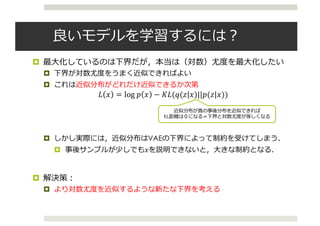
![実験:⽋損補間
¤ テストデータの⽋損補間
¤ 各例の右端が元画像
ed as a conference paper at ICLR 2016
(a) (b) (c)
5: (a) The samples generated from VAE-DGP trained on the combination of Frey faces and
ces (Frey-Yale). (b) Imputation from the test set of Frey-Yale. (c) Imputation from the test
VHN. The gray color indicates the missing area. The 1st column shows the input images,
column show the imputed images and 3rd column shows the original full images.
KF1F1 , KU1U1 are the covariance matrices of F1 and U1 respectively, KF1U1 is the cross-
nce matrix between F1 and U1, and 1 = Tr(hKF1F1 iq(X1)), 1 = hKF1U1 iq(X1) and
⌦
K>
F1U1
KF1U1
↵
q(X )
, and ⇤1 = KU1U1
+ 1. This enables data-parallelism by dis-
Published as a conference paper at ICLR 2016
5.1 UNSUPERVISED LEARNING
Model MNIST
DBN 138±2
Stacked CAE 121 ± 1.6
Deep GSN 214 ± 1.1
Adversarial nets 225 ± 2
GMMN+AE 282 ± 2
VAE-DGP (5) 301.67
VAE-DGP (10-50) 674.86
VAE-DGP (5-20-50) 723.65
Table 1: Log-likelihood for the MNIST test
data with different models. The baselines are
DBN and Stacked CAE (Bengio et al., 2013),
Deep GSN (Bengio et al., 2014), Adversarial
nets (Goodfellow et al., 2014) and GMMN+AE
(Li et al., 2015).
Figure 6: Samples of imputation on the test
sets. The gray color indicates the missing
area. The 1st column shows the input im-
ages, the 2nd column show the imputed im-
ages and 3rd column shows the original full
images.
We first apply to our model to the combination of Frey faces and Yale faces (Frey-Yale). The Frey
faces contains 1956 20 ⇥ 28 frames taken from a video clip. The Yale faces contains 2414 images,
which are resized to 20 ⇥ 28. We take the last 200 frames from the Frey faces and 300 images
randomly from Yale faces as the test set and use the rest for training. The intensity of the original
gray-scale images are normalized to [0, 1]. The applied VAE-DGP has two hidden layers (a 2D top
hidden layer and a 20D middle hidden layer). The exponentiated quadratic kernel is used for all the
layers with 100 inducing points. All the MLPs in the recognition model have two hidden layers with](https://image.slidesharecdn.com/iclr2016vae-160920054645/85/Iclr2016-vae-29-320.jpg)
![実験:精度評価
¤ 対数尤度(MNIST)
¤ 教師あり学習(回帰)
¤ データセット:
¤ The Abalone dataset
¤ The Creep dataset
Published as a conference paper at ICLR 2016
5.1 UNSUPERVISED LEARNING
Model MNIST
DBN 138±2
Stacked CAE 121 ± 1.6
Deep GSN 214 ± 1.1
Adversarial nets 225 ± 2
GMMN+AE 282 ± 2
VAE-DGP (5) 301.67
VAE-DGP (10-50) 674.86
VAE-DGP (5-20-50) 723.65
Table 1: Log-likelihood for the MNIST test
data with different models. The baselines are
DBN and Stacked CAE (Bengio et al., 2013),
Deep GSN (Bengio et al., 2014), Adversarial
nets (Goodfellow et al., 2014) and GMMN+AE
(Li et al., 2015).
Figure 6: Samples of imputation on the test
sets. The gray color indicates the missing
area. The 1st column shows the input im-
ages, the 2nd column show the imputed im-
ages and 3rd column shows the original full
images.
We first apply to our model to the combination of Frey faces and Yale faces (Frey-Yale). The Frey
faces contains 1956 20 ⇥ 28 frames taken from a video clip. The Yale faces contains 2414 images,
which are resized to 20 ⇥ 28. We take the last 200 frames from the Frey faces and 300 images
randomly from Yale faces as the test set and use the rest for training. The intensity of the original
gray-scale images are normalized to [0, 1]. The applied VAE-DGP has two hidden layers (a 2D top
hidden layer and a 20D middle hidden layer). The exponentiated quadratic kernel is used for all the
layers with 100 inducing points. All the MLPs in the recognition model have two hidden layers with
widths (500-300). As a generative model, we can draw samples from the learned model by sampling
first from the prior distribution of the top hidden layer (a 2D unit Gaussian distribution in this case)
and layer-wise downwards. The generated images are shown in Figure 5a.
To evaluate the ability of our model learning the data distribution, we train the VAE-DGP on MNIST
(LeCun et al., 1998). We use the whole training set for learning, which consists of 60,000 28 ⇥ 28
images. The intensity of the original gray-scale images are normalized to [0, 1]. We train our model
with three different model settings (one, two and three hidden layers). The trained models are
Published as a conference paper at ICLR 2016
Figure 7: Bayesian optimization experiments for
Model Abalone
VEA-DGP 825.31 ± 64.35
GP 888.96 ± 78.22
Lin. Reg. 917.31 ± 53.76
Model Creep
VEA-DGP 575.39 ± 29.10
GP 602.11 ± 29.59
Lin. Reg. 1865.76 ± 23.36
Table 2: MSE obtained from our VEA-DGP,
standard GP and linear regression for the
Abalone and Creep benchmarks.](https://image.slidesharecdn.com/iclr2016vae-160920054645/85/Iclr2016-vae-30-320.jpg)
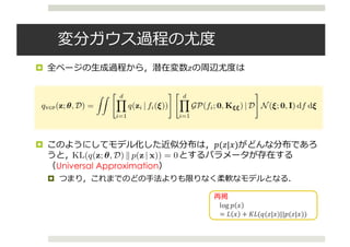
![変分推論における平均場近似
¤ VAEでは近似分布は𝑞(𝑧|𝑥)と考えてきた
¤ 𝑞(𝑧|𝑥)はニューラルネットワークで表現
¤ ⼀般的に近似分布は平均場近似によって近似される.
¤ もっとリッチな近似分布を考えることもできる
¤ パラメータ𝜆を確率変数として事前分布を考える(階層変分モデル)
log 𝑝 𝑥
= 𝐿 𝑥 + 𝐾𝐿(𝑞(𝑧|𝑥)||𝑝(𝑧|𝑥))
4
Variational Models
• We want to compute posterior p(z|x) (z: latent variables, x: data)
• Variational inference seeks to minimize
for a family q(z; )
KL(q(z; )||p(z|x))
• Maximizing evidence lower bound (ELBO)
log p(x) Eq(z; )[log p(x|z)] KL(q(z; )||p(z))
• (Common) Mean-field distribution q(z; ) =
Y
i
q(zi; i)
• Hierarchical variational models
• (Newer) Interpret the family as a variational model for posterior
latent variables z (introducing new latent variables)[1]
Lawrence, N. (2000). Variational Inference in Probabilistic Models. PhD thesis.](https://image.slidesharecdn.com/iclr2016vae-160920054645/85/Iclr2016-vae-31-320.jpg)
![変分ガウス過程
¤ The Variational Gaussain Process [Tran+ 15; ICLR 2016]
¤ とても強⼒な変分モデルを提案
¤ を変分データ(パラメータ)とし,次のような𝑧の
⽣成過程を考える.
¤ 潜在変数
¤ ⾮線形写像をDによって条件づけられたガウス過程から⽣成
¤ 潜在変数zを⽣成
7
Variational Gaussian Processes
7
Variational Gaussian Processes
Variational Gaussian Processes
7
Variational Gaussian Processes
Variational Gaussian Processes](https://image.slidesharecdn.com/iclr2016vae-160920054645/85/Iclr2016-vae-32-320.jpg)
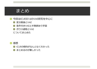
![下界
¤ 学習では次の下界を最⼤化する
¤ イメージとしては次のような感じ
¤ 近似モデルでxからzを⽣成
¤ 補助モデルでxとzから写像と潜在変数を⽣成
3 BLACK BOX INFERENCE
3.1 VARIATIONAL OBJECTIVE
We derive an algorithm for performing black box inference over a wide class of generative models.
The original ELBO (Eq.1) is analytically intractable due to the log density log qVGP(z) (Eq.4). We
derive a tractable variational objective inspired by auto-encoders.
Specifically, a tractable lower bound to the model evidence log p(x) can be derived by subtracting
an expected KL divergence term from the ELBO:
log p(x) EqVGP
[log p(x | z)] KL(qVGP(z)kp(z)) EqVGP
h
KL(q(⇠, f | z)kr(⇠, f | z))
i
,
where r(⇠, f | z) is an auxiliary model. Such an objective has been considered independently by Sal-
imans et al. (2015) and Ranganath et al. (2015). Variational inference is performed in the posterior
latent variable space, minimizing KL(qkp) to learn the variational model; for this to occur auxil-
iary inference is performed in the variational latent variable space, minimizing KL(qkr) to learn an
auxiliary model. See Figure 2.
Unlike previous approaches, we rewrite this variational objective to connect to auto-encoders:
eL = EqVGP
[log p(x | z)] EqVGP
h
KL(q(z | f(⇠))kp(z)) + KL(q(⇠, f)kr(⇠, f | z))
i
, (5)
where the KL divergences are now taken over tractable distributions (see Appendix C). In auto-
encoder parlance, we maximize the expected negative reconstruction error, regularized by an ex-
pected divergence between the variational model and the original model’s prior, and an expected
divergence between the auxiliary model and the variational model’s prior. This is simply a nested
instantiation of the variational auto-encoder bound (Kingma & Welling, 2014): a KL divergence
between the inference model and a prior is taken as regularizers on both the posterior and variational
spaces. This interpretation justifies the previously proposed bound for variational models; as we
shall see, it also enables lower variance gradients during stochastic optimization.
5
再構成誤差 正規化項
補助モデル
Under review as a conference paper at ICLR 2016
3.2 AUTO-ENCODING VARIATIONAL MODELS
Inference networks provide a flexible parameterization of approximating
in Helmholtz machines (Hinton & Zemel, 1994), deep Boltzmann machin
Larochelle, 2010), and variational auto-encoders (Kingma & Welling, 2014; R
replaces local variational parameters with global parameters coming from a ne
ically, for latent variables zn which correspond to a data point xn, an infere
a neural network which takes xn as input and its local variational parameter
amortizes inference by only defining a set of global parameters.
To auto-encode the VGP we specify inference networks to parameterize bo
auxiliary models. Unique from other auto-encoder approaches, we let the aux
observed data point xn and variational data point zn as input:
xn 7! q(zn | xn; ✓n), xn, zn 7! r(⇠n, fn | xn, zn; n
where q has local variational parameters given by the variational data Dn, a
fully factorized Gaussian with local variational parameters n = (µn 2 R
Note that by letting r’s inference network take both xn and zn as input, w
explicit specification of r(✏, f | z). This idea was first suggested but not imple
et al. (2015).
w as a conference paper at ICLR 2016
ENCODING VARIATIONAL MODELS
tworks provide a flexible parameterization of approximating distributions as used
z machines (Hinton & Zemel, 1994), deep Boltzmann machines (Salakhutdinov &
010), and variational auto-encoders (Kingma & Welling, 2014; Rezende et al., 2014). It
l variational parameters with global parameters coming from a neural network. Specif-
ent variables zn which correspond to a data point xn, an inference network specifies
work which takes xn as input and its local variational parameters n as output. This
erence by only defining a set of global parameters.
ode the VGP we specify inference networks to parameterize both the variational and
dels. Unique from other auto-encoder approaches, we let the auxiliary model take both
a point xn and variational data point zn as input:
xn 7! q(zn | xn; ✓n), xn, zn 7! r(⇠n, fn | xn, zn; n),
local variational parameters given by the variational data Dn, and r is specified as a
ed Gaussian with local variational parameters n = (µn 2 Rc+d
, 2
n 2 Rc+d
). 1
letting r’s inference network take both x and z as input, we avoid the restrictive](https://image.slidesharecdn.com/iclr2016vae-160920054645/85/Iclr2016-vae-34-320.jpg)
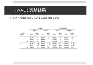
![実験:対数尤度
¤ 前⼈未到の70代に突⼊
¤ ⽣成部分のモデルをDRAW, 近似分布をVGPとしたモデルが⼀番良い
Published as a conference paper at ICLR 2016
Model log p(x)
DLGM + VAE [1] 86.76
DLGM + HVI (8 leapfrog steps) [2] 85.51 88.30
DLGM + NF (k = 80) [3] 85.10
EoNADE-5 2hl (128 orderings) [4] 84.68
DBN 2hl [5] 84.55
DARN 1hl [6] 84.13
Convolutional VAE + HVI [2] 81.94 83.49
DLGM 2hl + IWAE (k = 50) [1] 82.90
DRAW [7] 80.97
DLGM 1hl + VGP 84.79
DLGM 2hl + VGP 81.32
DRAW + VGP 79.88
Table 1: Negative predictive log-likelihood for binarized MNIST. Previous best results are
[1] (Burda et al., 2016), [2] (Salimans et al., 2015), [3] (Rezende & Mohamed, 2015), [4] (Raiko
et al., 2014), [5] (Murray & Salakhutdinov, 2009), [6] (Gregor et al., 2014), [7] (Gregor et al., 2015).](https://image.slidesharecdn.com/iclr2016vae-160920054645/85/Iclr2016-vae-35-320.jpg)

This document summarizes a presentation about variational autoencoders (VAEs) presented at the ICLR 2016 conference. The document discusses 5 VAE-related papers presented at ICLR 2016, including Importance Weighted Autoencoders, The Variational Fair Autoencoder, Generating Images from Captions with Attention, Variational Gaussian Process, and Variationally Auto-Encoded Deep Gaussian Processes. It also provides background on variational inference and VAEs, explaining how VAEs use neural networks to model probability distributions and maximize a lower bound on the log likelihood.


![[DL輪読会]相互情報量最大化による表現学習](https://cdn.slidesharecdn.com/ss_thumbnails/20190913iwasawa-190913002312-thumbnail.jpg?width=640&height=640&fit=bounds)

![[DL輪読会]Recent Advances in Autoencoder-Based Representation Learning](https://cdn.slidesharecdn.com/ss_thumbnails/20190119dljournalclubweb-190401063633-thumbnail.jpg?width=640&height=640&fit=bounds)


![[DL輪読会]data2vec: A General Framework for Self-supervised Learning in Speech,...](https://cdn.slidesharecdn.com/ss_thumbnails/220204nonakadl1-220204025334-thumbnail.jpg?width=640&height=640&fit=bounds)


![[DL輪読会]GQNと関連研究,世界モデルとの関係について](https://cdn.slidesharecdn.com/ss_thumbnails/20180817-180827085537-thumbnail.jpg?width=640&height=640&fit=bounds)

![[DL輪読会]NVAE: A Deep Hierarchical Variational Autoencoder](https://cdn.slidesharecdn.com/ss_thumbnails/nvaeadeephierarchicalvariationalautoencoder-201113004930-thumbnail.jpg?width=640&height=640&fit=bounds)


![[DL輪読会]Generative Models of Visually Grounded Imagination](https://cdn.slidesharecdn.com/ss_thumbnails/20170602-170602005505-thumbnail.jpg?width=640&height=640&fit=bounds)