Downloaded 123 times

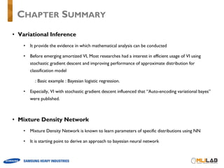
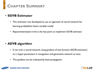
![• Supervised learning
e.g) Bayesian logistic regression
𝑝 𝑥 𝑤, 𝑦 ⋅ 𝑝 𝑤 ∝ 𝑝 𝑤, 𝑥 𝑦
𝑝 𝑥 𝑤, 𝑦 ∶ ∏ 𝜎 𝑤R
𝑥 ST ⋅ (1 − 𝜎 𝑤R
𝑥 %VST).
W1% à Approximate Gaussian Dist.
• Latent Variable Model
e.g) Gaussian Mixture Model (EM algorithm)
à tractable conditional pdf : 𝑝(𝑧|𝑥)
𝑞 𝑧 ≈ 𝑝 𝑧 𝑥, 𝜃Z[
𝜃∗
= 𝑎𝑟𝑔𝑚𝑎𝑥] ^ 𝑝 𝑧 𝑥, 𝜃Z[
⋅ 𝑙𝑛𝑝(𝑥, 𝑧|𝜃)
_
PROBABILITY GRAPHICAL MODEL](https://image.slidesharecdn.com/180921isanyoneinterestinauto-encodingvariational-bayes-181127055600/85/is-anyone_interest_in_auto-encoding_variational-bayes-10-320.jpg)
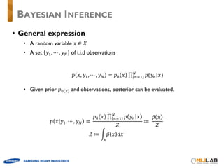
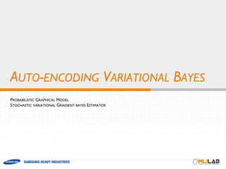
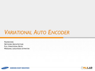
![• Mean field assumption
• If 𝑝(𝑧|𝑥) is intractable ?
𝑞 𝒛 = a 𝑞W(𝑧W)
W
𝑙𝑛𝑞b
∗
𝑧b = 𝐸Wdb 𝑙𝑛𝑝 𝒙, 𝒛 + 𝑐𝑜𝑛𝑠𝑡
𝑞b
∗
𝑧b =
exp ( 𝐸Wdb[𝑙𝑛𝑝 𝒙, 𝒛 ]
∫ exp ( 𝐸Wdb 𝑙𝑛𝑝 𝒙, 𝒛 𝑑𝑧
• Under specific probabilistic graphical model, approximate distribution can be evaluated by
expectation of 𝐸Wdb[𝑙𝑛𝑝 𝒙, 𝒛 ]
• Depending on each problem, we have to derive the form of 𝐸Wdb[𝑙𝑛𝑝 𝒙, 𝒛 ]
• Through sequential optimization, All of 𝑞b(𝑧b) can be updated in order until converged.
TRADITIONAL VARIATIONAL INFERENCE](https://image.slidesharecdn.com/180921isanyoneinterestinauto-encodingvariational-bayes-181127055600/85/is-anyone_interest_in_auto-encoding_variational-bayes-11-320.jpg)
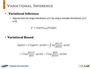
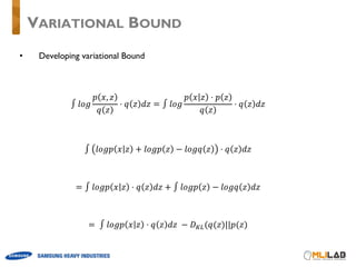
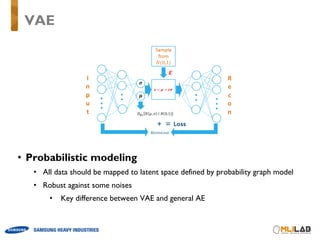
![• VI with Stochastic gradient descent
𝐿 = ∫ 𝑙𝑜𝑔
𝑝 𝑥, 𝑧
𝑞o 𝑧
⋅ 𝑞o 𝑧 𝑑𝑧
𝛻o 𝐿 = ∫ 𝑙𝑛𝑝 𝑥, 𝑧 ⋅ 𝛻o 𝑙𝑛𝑞 𝑧 ⋅ 𝑞 𝑧 𝑑𝑧 = 𝐸2∼C[𝑙𝑛𝑝 𝑥, 𝑧 ⋅ 𝛻o 𝑙𝑛𝑞 𝑧 ]
𝛻o 𝐿 = 𝐸2∼C 𝑙𝑛𝑝 𝑥, 𝑧 ⋅ 𝛻o 𝑙𝑛𝑞 𝑧 ≈
1
𝑛
^ 𝑙𝑛𝑝 𝑥W, 𝑧
W
⋅ 𝛻o 𝑙𝑛𝑞 𝑧
• In order to avoid exact derivation of expectation and sequential optimization, stochastic
gradient descent method was introduced.
• This method only requires 𝑙𝑜𝑔𝑝 𝑥, 𝑧 , 𝑞o 𝑧 and its derivative
• All components can be easily handed
• 𝑙𝑜𝑔𝑝 𝑥, 𝑧 can be derived from probabilistic graphical model
• 𝑞o 𝑧 and 𝛻o 𝑞o 𝑧 are decided by users.
• However, since this estimator has a huge variance, it also requires many samples.
TRADITIONAL VARIATIONAL INFERENCE (2)](https://image.slidesharecdn.com/180921isanyoneinterestinauto-encodingvariational-bayes-181127055600/85/is-anyone_interest_in_auto-encoding_variational-bayes-12-320.jpg)
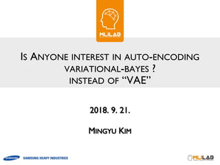
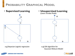
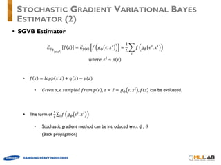
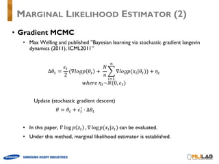
![• Mixture density network
• 𝑝 𝑥 𝑤, 𝑦 ⋅ 𝑝 𝑤 ∝ 𝑝 𝑤, 𝑥 𝑦
𝐸 𝑤 = − ^ ln { ^ 𝜋v 𝑥., 𝑤 𝑁(𝑡.|𝑢v 𝑥., 𝑤 , 𝜎v
y
𝑥., 𝑤 )}
{
v1%
(
.1%
Mixture density network presents that artificial neural network trains hyper-parameters for
learning parameters of distributions
NETWORK FOR LEARNING PARAMETERS
[ Structure of Mixture density Network ] [ Data point and result by Mixture Density Network]](https://image.slidesharecdn.com/180921isanyoneinterestinauto-encodingvariational-bayes-181127055600/85/is-anyone_interest_in_auto-encoding_variational-bayes-13-320.jpg)
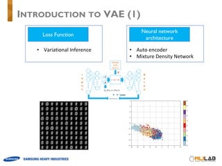
![• Amortized generative model
• 𝜙 : hyper-parameters in recognition network
• 𝜃 : hyper-parameters in generative network
PROBABILISTIC GRAPHICAL MODEL
NX
Z
𝜙 𝜃
p
𝜇 𝜎
NX
Z
𝜃
𝜙
Generative model
Variational
approximation
[ AEVB algorithm ] [ VAE ]](https://image.slidesharecdn.com/180921isanyoneinterestinauto-encodingvariational-bayes-181127055600/85/is-anyone_interest_in_auto-encoding_variational-bayes-16-320.jpg)
![• Traditional Latent variable model
• Intractable : 𝑝(𝑧|𝑥)
• A large data set : Sampling based EM algorithm à Too slow
• This paper has interested in
• Using stochastic gradient descent
• Efficient approximate posterior inference of latent variable 𝑧
• This paper introduce (The reason why this method referred ”Variational”)
• 𝑞o 𝑧 𝑥 : recognition model / approximate posterior distribution to 𝑝] 𝑧 𝑥
• Figure out parameters of approximate distribution
• 𝑝] 𝑥 𝑧 : generative model (defined as graphical model)
• Learning the recognition model parameter 𝜙 with generative model parameter 𝜃
using reparameterization trick
PROBLEMS SCENARIO](https://image.slidesharecdn.com/180921isanyoneinterestinauto-encodingvariational-bayes-181127055600/85/is-anyone_interest_in_auto-encoding_variational-bayes-17-320.jpg)
![• Reparametrization Trick
• Random variable z à Function of variables (Deterministic)
• Capable of using neural network
• 𝑧 ~ 𝑞 𝑧 𝑥 à 𝑧̅ = 𝑔o(𝑥, ϵ), 𝜖 ~ 𝑝 𝜖
• Assume that 𝑝 𝜖 is defined (𝑝 𝜖 ~ 𝑁(0,1))
• The function 𝑔] is determined depending on 𝑞 𝑧 𝑥
(In subsequent chapter, the forms of function 𝑔] is represented)
• Form of function 𝑔]
• Tractable inverse CDF : similar to finding PDF
• 𝐹 𝑥 = 𝑝, 𝐹V%
𝑝 = 𝑥 𝑢𝑛𝑖𝑞𝑢𝑒 𝑥 / 𝑔o 𝜖, 𝑥 = Fo
V%
𝜖; 𝑥 = 𝑍̅
• Location Scale Model :
• 𝑔o 𝜖, 𝑥 = location + scale ⋅ 𝜖
STOCHASTIC GRADIENT VARIATIONAL BAYES
ESTIMATOR (1)](https://image.slidesharecdn.com/180921isanyoneinterestinauto-encodingvariational-bayes-181127055600/85/is-anyone_interest_in_auto-encoding_variational-bayes-19-320.jpg)
![• SGVB Estimator A
𝐿’“(𝜃, 𝜙; 𝑥W
) =
1
𝐿
^ 𝑙𝑜𝑔𝑝 ] 𝑥W
, 𝑧W,[
− 𝑙𝑜𝑔𝑞o(𝑧W,[
|𝑥W
)
[
𝑤ℎ𝑒𝑟𝑒, 𝑔o 𝜖, 𝑥W
, 𝜖[
~ 𝑝 𝜖
• 𝑙𝑜𝑔𝑝 ] 𝑥W
, 𝑧W,[
is defined by probabilistic graphical model
• 𝑙𝑜𝑔𝑞o(𝑧W,[
|𝑥W
) can be determined 𝑔o 𝜖, 𝑥W
, 𝜖[
~ 𝑝 𝜖
• SGVB Estimator B
𝐿”“(𝜃, 𝜙; 𝑥W
) =
1
𝐿
^ 𝑙𝑜𝑔𝑝 ] 𝑥W
|𝑧W,[
− 𝐷{•(𝑞o(𝑧|𝑥W
)||𝑝] 𝑧 )
[
𝑤ℎ𝑒𝑟𝑒, 𝑔o 𝜖, 𝑥W
, 𝜖[
~ 𝑝 𝜖
• 𝐷{•(𝑞o(𝑧|𝑥W
)||𝑝] 𝑧 ) is analytically evaluated (Gaussian Dist.)
• 𝐷{•(𝑞o(𝑧|𝑥W
)||𝑝] 𝑧 ) doesn’t require sample z, only require parameter of approximate dist.
STOCHASTIC GRADIENT VARIATIONAL BAYES
ESTIMATOR (3)](https://image.slidesharecdn.com/180921isanyoneinterestinauto-encodingvariational-bayes-181127055600/85/is-anyone_interest_in_auto-encoding_variational-bayes-21-320.jpg)
![𝑙𝑛𝑝] 𝑋, 𝑍 = ^ 𝑙𝑛𝑝](𝑥W
|𝑧W
)
W
𝑙𝑛𝑞o 𝑍 = ^ 𝑙𝑛𝑞o(𝑧W
)
W
𝑙𝑛𝑝] 𝑍 = ^ 𝑙𝑛𝑝](𝑧W
)
W
AUTO ENCODING VARIATIONAL BAYES
ALGORITHM(1)
NX
Z𝜙 𝜃](https://image.slidesharecdn.com/180921isanyoneinterestinauto-encodingvariational-bayes-181127055600/85/is-anyone_interest_in_auto-encoding_variational-bayes-22-320.jpg)
![AUTO ENCODING VARIATIONAL BAYES
ALGORITHM (2)
• AEVB for SGVB estimator
1
𝑀
^ 𝐿’“(𝜃, 𝜙; 𝑥W
)
W
=
1
𝑀
^
1
𝐿
^ 𝑙𝑜𝑔𝑝 ] 𝑥W
, 𝑧W,[
− 𝑙𝑜𝑔𝑞o(𝑧W,[
|𝑥W
)
[
W
1
𝑀
^ 𝐿”“(𝜃, 𝜙; 𝑥W
)
W
=
1
𝑀
^
1
𝐿
^ 𝑙𝑜𝑔𝑝 ] 𝑥W
|𝑧W,[
− 𝐷{•(𝑞o(𝑧|𝑥W
)||𝑝] 𝑧 )
[W](https://image.slidesharecdn.com/180921isanyoneinterestinauto-encodingvariational-bayes-181127055600/85/is-anyone_interest_in_auto-encoding_variational-bayes-23-320.jpg)
![• Loss function (Bernoulli Case)
• 𝑝 𝑧 ~ 𝑁(0, 𝐼)
• 𝑝] 𝑥|𝑧 ~ 𝑁 𝑢] 𝑧 , 𝜎] 𝑧 𝑜𝑟 𝐵𝑒𝑟𝑛(p] 𝑧 )
• 𝑞o 𝑧|𝑥 ~ 𝑁(𝑢o(𝑥), 𝑑𝑖𝑎𝑔o(𝑥))
• Estimator (Loss function)
𝐿”“(𝜃, 𝜙; 𝑥W
) =
1
𝐿
^ 𝑙𝑜𝑔𝑝 ] 𝑥W
|𝑧W,[
− 𝐷{•(𝑞o(𝑧|𝑥W
)||𝑝] 𝑧 )
[
𝑤ℎ𝑒𝑟𝑒 𝑔o 𝜖, 𝑥W
= 𝑢] 𝑥 + 𝜖 ⋅ 𝜎] 𝑥
𝜖 ~ 𝑁 0, 𝐼 , 𝑙 = 1
• Since 𝑙 = 1, neural network architecture can be similar to “auto-encoder”
FRAMEWORK (1)](https://image.slidesharecdn.com/180921isanyoneinterestinauto-encodingvariational-bayes-181127055600/85/is-anyone_interest_in_auto-encoding_variational-bayes-26-320.jpg)
![• Loss function
• 𝑝] 𝑥|𝑧 ~ 𝐵𝑒𝑟𝑛 p] 𝑧
à 𝑙𝑜𝑔𝑝] 𝑥|𝑧 ~ ∑ 𝑥W 𝑙𝑜𝑔pW ]
𝑧W + 1 − 𝑥W 𝑙𝑜𝑔(1 − p](𝑧W))
• 𝐷{•(𝑞o(𝑧|𝑥W)||𝑝] 𝑧 )
• 𝑝 𝑧 ~ 𝑁 0, 𝐼 , 𝑞o 𝑧|𝑥 ~ 𝑁(𝑢o(𝑥), 𝑑𝑖𝑎𝑔o(𝑥))
• 𝐷{•(𝑞o(𝑧|𝑥)| 𝑝] 𝑧 =
%
y
{ 0 − 𝑢o 𝑥 𝐼V% 0 − 𝑢o 𝑥 + 𝑡𝑟𝑎𝑐𝑒(𝐼V% 𝑑𝑖𝑎𝑔o(𝑥)) − 𝑘 + 𝑙𝑛
|™|
|Wš›ˆ 2 |
= ^ 𝑢o 𝑥 (b)
y
− 1 + 𝜎o
y
𝑥 b − 𝑙𝑛𝜎o
y
𝑥 (b)
b
𝑤ℎ𝑒𝑟𝑒 𝑗 = 𝑖𝑛𝑑𝑒𝑥 𝑜𝑓 𝑑𝑖𝑚𝑒𝑛𝑠𝑖𝑜𝑛 𝑜𝑓 𝑙𝑎𝑡𝑒𝑛𝑡 𝑣𝑎𝑟𝑖𝑎𝑏𝑙𝑒 𝑧
FRAMEWORK (2)](https://image.slidesharecdn.com/180921isanyoneinterestinauto-encodingvariational-bayes-181127055600/85/is-anyone_interest_in_auto-encoding_variational-bayes-27-320.jpg)
![• Loss Function
∴ ∑ 𝑥W 𝑙𝑜𝑔pW ]
𝑧W + 1 − 𝑥W 𝑙𝑜𝑔(1 − p](𝑧W)) +
^ ^ 𝑢o 𝑥W (b)
y
− 1 + 𝜎o
y
𝑥W b − 𝑙𝑛𝜎o
y
𝑥W (b)
bW
FRAMEWORK (3)](https://image.slidesharecdn.com/180921isanyoneinterestinauto-encodingvariational-bayes-181127055600/85/is-anyone_interest_in_auto-encoding_variational-bayes-28-320.jpg)
![• Network Architecture
• Recognition network (like density network)
𝑢o 𝑥W = 𝑤y 𝑡𝑎𝑛ℎ 𝑤% 𝑥W + 𝑏% + 𝑏y
𝜎o 𝑥W = 𝑤Ÿ 𝑡𝑎𝑛ℎ 𝑤 𝑥W + 𝑏 + 𝑏Ÿ
• Generative network
• Bernoulli Case
p] 𝑧W = 𝑓š 𝑤y tanh 𝑤% 𝑧W + 𝑏% + 𝑏y
𝑤ℎ𝑒𝑟𝑒 𝑓š ⋅ : 𝑒𝑙𝑒𝑚𝑒𝑛𝑡 − 𝑤𝑖𝑠𝑒 𝑠𝑖𝑔𝑚𝑜𝑖𝑑 𝑓𝑢𝑛𝑐𝑡𝑖𝑜𝑛
𝜃 = {𝑤%, 𝑏%, 𝑤y, 𝑏y}
• Gaussian Case
𝑢] 𝑧W = 𝑤Ÿ(𝑡𝑎𝑛ℎ 𝑤 𝑧 + 𝑏 + 𝑏Ÿ
𝜎] 𝑧W = 𝑤¥(𝑡𝑎𝑛ℎ 𝑤 𝑧 + 𝑏 + 𝑏¥
𝜃 = {𝑤 , 𝑤Ÿ, 𝑤¥, 𝑏 , 𝑏Ÿ, 𝑏¥}
STRUCTURE OF VAE(1)](https://image.slidesharecdn.com/180921isanyoneinterestinauto-encodingvariational-bayes-181127055600/85/is-anyone_interest_in_auto-encoding_variational-bayes-29-320.jpg)
![• Derivation
• Marginal Likelihood : 𝑝 ] (𝑥)
• Marginal likelihood estimator
1
𝑝](𝑥W)
= ∫
𝑞 𝑧
𝑝] 𝑥W
𝑑𝑧 =
∫ 𝑞 𝑧 ⋅
𝑝] 𝑥W, 𝑧
𝑝] 𝑥W, 𝑧
𝑑𝑧
𝑝] 𝑥W
= ∫
𝑝] 𝑥W, 𝑧
𝑝] 𝑥W
⋅
𝑞 𝑧
𝑝] 𝑥W, 𝑧
𝑑𝑧
= ∫ 𝑝] 𝑧 𝑥W
𝑞 𝑧
𝑝] 𝑥W, 𝑧
𝑑𝑧 ≈
1
𝐿
^
𝑞o(𝑧 [
)
𝑝] 𝑧 𝑝](𝑥W|𝑧 [ )
[
• In VAE, marginal likelihood estimator cannot be evaluated
because it requires 𝑙 > 1
• If it was forced to evaluate the marginal likelihood in VAE, the result is almost same
as loss function, it doesn’t give any special meaning.
MARGINAL LIKELIHOOD ESTIMATOR (1)](https://image.slidesharecdn.com/180921isanyoneinterestinauto-encodingvariational-bayes-181127055600/85/is-anyone_interest_in_auto-encoding_variational-bayes-31-320.jpg)
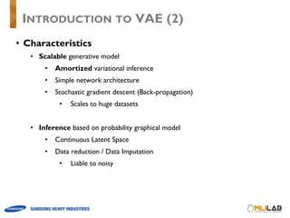
![• Framework
• 𝑝] 𝑧 ~ 𝑁 0, 𝐼 , 𝑤ℎ𝑒𝑟𝑒 𝑧 ∈ 𝑅°, 𝐼 ∈ 𝑅°×°
• 𝑝² 𝜃 ~ 𝑁 0, 𝐼 , 𝑤ℎ𝑒𝑟𝑒 𝜃 ∈ 𝑅³, 𝐼 ∈ 𝑅³×³
• 𝑝] 𝑥|𝑧 ~ 𝑁 𝑢] 𝑧 , 𝜎] 𝑧 𝑜𝑟 𝐵𝑒𝑟𝑛(p] 𝑧 )
• 𝑞o 𝑧|𝑥 ~ 𝑁(𝑢o(𝑥), 𝑑𝑖𝑎𝑔o(𝑥))
FULL VARIATIONAL BAYES
NX
Z
𝜙 𝜃
[ AEVB algorithm ]
𝛼](https://image.slidesharecdn.com/180921isanyoneinterestinauto-encodingvariational-bayes-181127055600/85/is-anyone_interest_in_auto-encoding_variational-bayes-33-320.jpg)
![• Variational Bound
𝑙𝑛𝑝] 𝑋 ≈ ∫ 𝑙𝑛𝑃² 𝑋 𝜃 + 𝑙𝑛𝑃² 𝜃 − 𝑙𝑛𝑞o 𝜃 ⋅ 𝑞] 𝜃 𝑑𝜃
=
1
𝐿
^ 𝐸 𝑙𝑛𝑃² 𝑋 𝜃 +
1
2
^{1 + 𝑙𝑛𝜎]
y
[
− 𝜇]
y
[
³
³1%
−𝜎]·
y ([)
}
•
[1%
𝑙𝑛𝑃² 𝑋 𝜃 = ∫ 𝑙𝑜𝑔
𝑝 𝑥, 𝑧
𝑞 𝑧
⋅ 𝑞 𝑧 𝑑𝑧 − ∫ 𝑙𝑜𝑔
𝑞 𝑧
𝑝 𝑧 𝑥
⋅ 𝑞 𝑧 𝑑𝑧
≈
1
𝐾
^(
(
W1%
^ ln𝑝] 𝑥W 𝑧W,b +
1
2
{
v1%
^{1 + 𝑙𝑛𝜎_
y
W,b
v
− 𝜇_
y
W,b
v
°
b1%
−𝜎_T,b
y (v)
})
• In this paper, 𝐿 = 𝐾 = 1 and ln𝑝] 𝑥W 𝑧W,b = 𝑙𝑛𝑝](𝑥|𝑧) , ∀𝑥W
∴ 𝑁 ⋅ 𝑙𝑛𝑝 𝑥 𝑧 +
𝑁
2
⋅ ^{1 + 𝑙𝑛𝜎_
y
W,b
¬
− 𝜇_
y
W,b
¬
°
b1%
−𝜎_T,b
y ¬
} +
1
2
^{1 + 𝑙𝑛𝜎]
y
[
− 𝜇]
y
[
³
³1%
−𝜎]·
y ([)
}
FULL VARIATIONAL BAYES](https://image.slidesharecdn.com/180921isanyoneinterestinauto-encodingvariational-bayes-181127055600/85/is-anyone_interest_in_auto-encoding_variational-bayes-34-320.jpg)

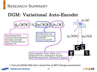


The document discusses auto-encoding variational Bayes (VAE), detailing its key concepts such as loss function, neural network architecture, and variational inference. It covers the reparameterization trick, stochastic gradient variational Bayes estimators, and provides insights on how these methods enhance posterior inference and scalability for large datasets. It also envelops a variety of applications and theoretical underpinnings that support the implementation of VAE in generative modeling.


![[기초개념] Graph Convolutional Network (GCN)](https://cdn.slidesharecdn.com/ss_thumbnails/agistdkimgcn190507-190507153736-thumbnail.jpg?width=640&height=640&fit=bounds)


![[DL輪読会]Recent Advances in Autoencoder-Based Representation Learning](https://cdn.slidesharecdn.com/ss_thumbnails/20190119dljournalclubweb-190401063633-thumbnail.jpg?width=640&height=640&fit=bounds)


![5G Explained! A High Level Overview [Introduction]](https://cdn.slidesharecdn.com/ss_thumbnails/5gexplainedahighleveloverview-260119165306-cc137a3e-thumbnail.jpg?width=640&height=640&fit=bounds)


