Download to read offline

![2. Methodology
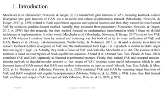
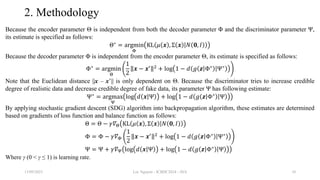
Note that ||x – x’|| is Euclidean distance between x and x’ whereas KL(μ(x), Σ(x) | N(0, I)) is Kullback-Leibler
divergence between Gaussian distribution of x whose mean vector and covariance matrix are μ(x) and Σ(x) and
standard Gaussian distribution N(0, I) whose mean vector and covariance matrix are 0 and identity matrix I.
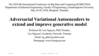
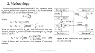
GAN developed by Goodfellow et al. (Goodfellow, et al., 2014) does not concern the encoder f(x | Θ) = z but
it focuses on optimizing the decoder g(z | Φ) = x’ by introducing a so-called discriminator which is a
discrimination function d(x | Ψ): x → [0, 1] from concerned data x or x’ to range [0, 1] in which d(x | Ψ) can
distinguish fake data from real data. In other words, the larger result the discriminator d(x’ | Ψ) derives, the more
realistic the generated data x’ is. Obviously, d(x | Ψ) is implemented by a DNN whose weights are Ψ with note
that this DNN has only one output neuron denoted d0. The essence of GAN is to optimize mutually the following
target function for estimating the decoder parameter Φ and the discriminator parameter Ψ (Goodfellow, et al.,
2014, p. 3).
𝑏GAN Φ, Ψ = log 𝑑 𝒙 Ψ + log 1 − 𝑑 𝑔 𝒛 Φ Ψ 2
Such that Φ and Ψ are optimized mutually as follows:
Φ∗
= argmin
Φ
𝑏GAN Φ, Ψ∗
Ψ∗
= argmax
Ψ
𝑏GAN Φ∗
, Ψ
13/09/2023 Loc Nguyen - ICBDC2024 - AVA 8](https://image.slidesharecdn.com/ava-icbdc2024-240601111212-b6aa6e1d/85/Adversarial-Variational-Autoencoders-to-extend-and-improve-generative-model-ICBDC2024-8-320.jpg)
![2. Methodology
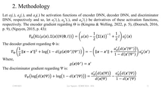
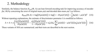
As a result, SGD algorithm incorporated into backpropagation algorithm for solving AVA is totally determined as
follows:
Θ = Θ − 𝛾 𝜇 𝒙 −
1
2
Σ 𝒙
−1
+
1
2
𝐼 𝑎𝑓
′
𝒙 5
Φ 𝑖 = Φ 𝑖 + 𝛾 𝒙 𝑖 − 𝒙′
𝑖 +
𝑎𝑑
′
𝑑 𝒙′
Ψ∗
1 − 𝑑 𝒙′
Ψ∗ 𝑎𝑔
′
𝒙′
𝑖 6
Ψ = Ψ + 𝛾
𝑎𝑑
′
𝑑 𝒙 Ψ
𝑑 𝒙 Ψ
−
𝑎𝑑
′
𝑑 𝒙′
Ψ
1 − 𝑑 𝒙′
Ψ
7
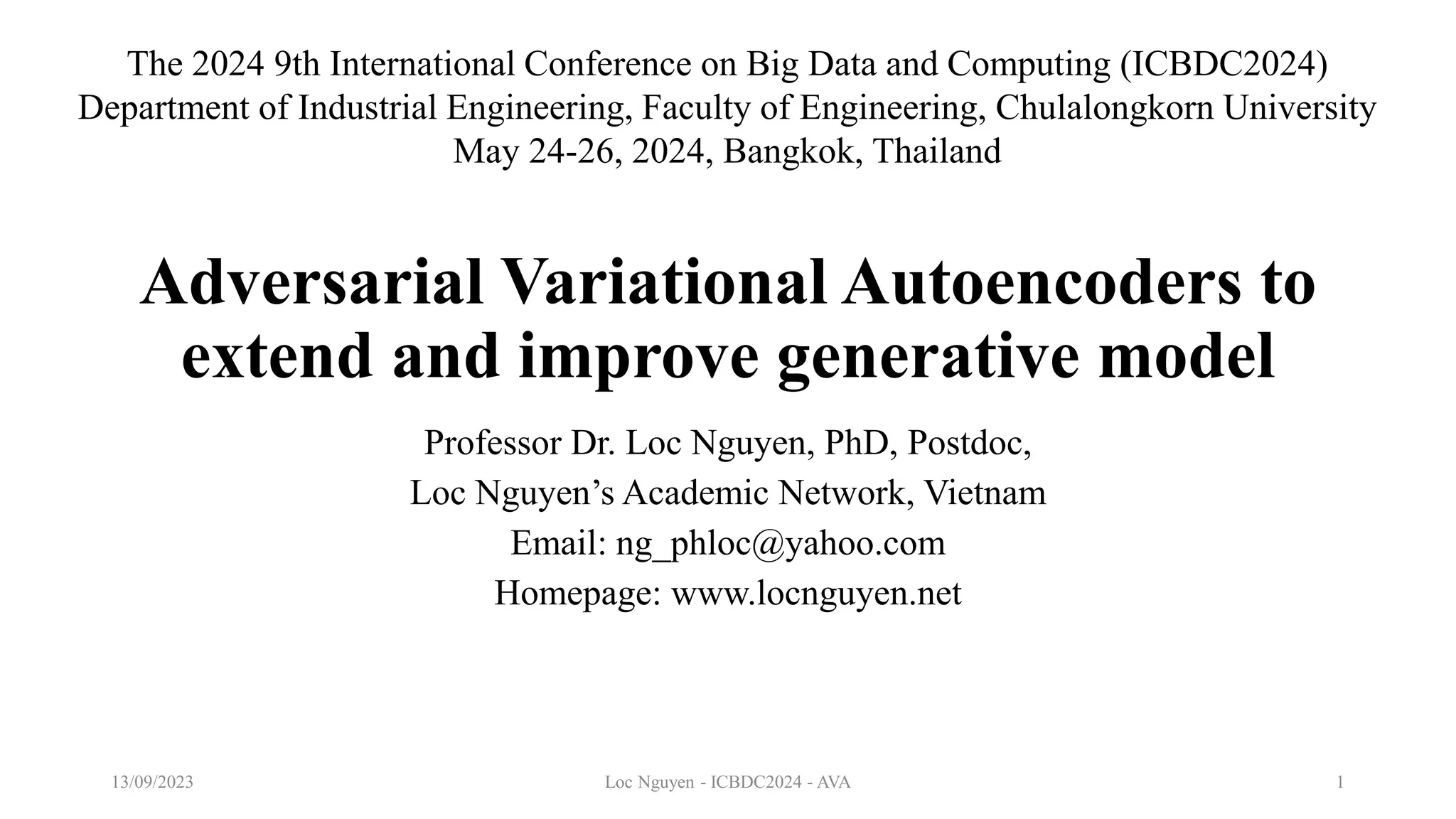
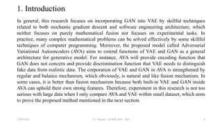
Where notation [i] denotes the ith element in vector. Please pay attention to the derivatives af’(.), ag’(.), and ad’(.) because
they are helpful techniques to consolidate AVA. The reason of two different occurrences of derivatives ad’(d(x’ | Ψ*)) and
ag’(x’) in decoder gradient regarding Φ is nontrivial because the unique output neuron of discriminator DNN is
considered as effect of the output layer of all output neurons in decoder DNN. When weights are assumed to be 1, error
of causal decoder neuron is error of discriminator neuron multiplied with derivative at the decoder neuron and moreover,
the error of discriminator neuron, in turn, is product of its minus bias –d’(.) and its derivative a’d(.) where d’(.) is
derivative of discriminator indeed.
error 𝒙′
𝑖 = 1 ∗ error 𝑑0 𝑎𝑔
′
𝒙′
𝑖
error 𝑑0 = −𝑑′
𝑑0 𝑎𝑑
′
𝑑0
13/09/2023 Loc Nguyen - ICBDC2024 - AVA 12
Figure 1. Causality effect relationship between
decoder DNN and discriminator DNN](https://image.slidesharecdn.com/ava-icbdc2024-240601111212-b6aa6e1d/85/Adversarial-Variational-Autoencoders-to-extend-and-improve-generative-model-ICBDC2024-12-320.jpg)
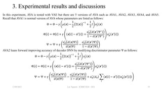
![2. Methodology
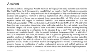
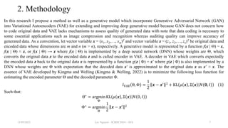
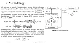
In a reverse causality effect relationship in which the unique output
neuron of discriminator DNN is cause of all output neurons of
decoder DNN as shown in figure 3.
Suppose bias of each decoder output neuron is bias[i], error of the
discriminator output neuron error[i] is sum of weighted biases which
is in turn multiplied with derivative at the discriminator output
neuron with note that every weighted bias is also multiplied with
derivative at every decoder output neuron. Suppose all weights are 1,
we have:
error 𝑖 = 𝑎𝑑
′
𝑑0
𝑖
bias 𝑖 𝑎𝑔
′
𝒙′
𝑖
bias 𝑖 = 𝒙 𝑖 − 𝒙′ 𝑖
13/09/2023 Loc Nguyen - ICBDC2024 - AVA 15
Figure 3. Reverse
causality effect
relationship
between
discriminator DNN
and decoder DNN](https://image.slidesharecdn.com/ava-icbdc2024-240601111212-b6aa6e1d/85/Adversarial-Variational-Autoencoders-to-extend-and-improve-generative-model-ICBDC2024-15-320.jpg)
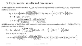
![2. Methodology
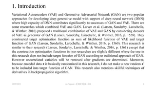
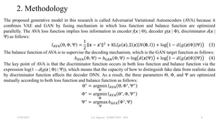
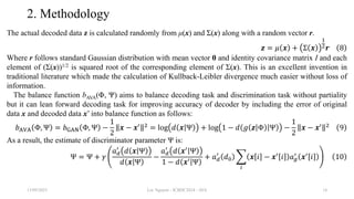
Because the balance function bAVA(Φ, Ψ) aims to improve the decoder g(z | Φ), it is possible to improve the encoder f(x
| Θ) by similar technique with note that output of encoder is mean vector μ(x) and covariance matrix Σ(x). In this
research, I propose another balance function BAVA(Θ, Λ) to assess reliability of the mean vector μ(x) because μ(x) is
most important to randomize z and μ(x) is linear. Let D(μ(x) | Λ) be discrimination function for encoder DNN from
μ(x) to range [0, 1] in which D(μ(x) | Λ) can distinguish fake mean μ(x’) from real mean μ(x). Obviously, D(μ(x) | Λ) is
implemented by a so-called encoding discriminator DNN whose weights are Λ with note that this DNN has only one
output neuron denoted D0. The balance function BAVA(Θ, Λ) is specified as follows:
𝐵AVA Θ, Λ = log 𝐷 𝜇 𝒙 Λ + log 1 − 𝐷 𝜇 𝒙′
Λ 11
Note,
𝑔 𝒛 Φ = 𝒙′
AVA loss function is modified with regard to the balance function BAVA(Θ, Λ) as follows:
𝑙AVA Θ, Φ, Ψ, Λ =
1
2
𝒙 − 𝒙′ 2
+ KL 𝜇 𝒙 , Σ 𝒙 𝑁 𝟎, 𝐼 + log 1 − 𝑑 𝒙′
Ψ + log 1 − 𝐷 𝜇 𝒙′
Λ 12
By similar way of applying SGD algorithm, it is easy to estimate the encoding discriminator parameter Λ as follows:
Λ = Λ + 𝛾
𝑎𝐷
′
𝐷 𝜇 𝒙 Λ
𝐷 𝜇 𝒙 Λ
−
𝑎𝐷
′
𝐷 𝜇 𝒙′
Λ
1 − 𝐷 𝜇 𝒙′
Λ
13
Where aD(.) and a’D(.) are activation function of the discriminator D(μ(x) | Λ) and its derivative, respectively.
13/09/2023 Loc Nguyen - ICBDC2024 - AVA 16](https://image.slidesharecdn.com/ava-icbdc2024-240601111212-b6aa6e1d/85/Adversarial-Variational-Autoencoders-to-extend-and-improve-generative-model-ICBDC2024-16-320.jpg)
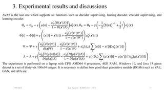
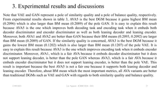
![3. Experimental results and discussions
Let imageGen be the best image generated by a deep generative model (DGM), which is compared with
the ith image denoted images[i] in dataset and then, let dij be the pixel distance between imageGen and
the ith image at the jth pixel as follows:
𝑑𝑖𝑗 = imageGen 𝑗 − image 𝑖 𝑗
Obviously, image[i][j] (imageGen[j]) is the jth pixel of the ith image (the generated image). The notation
||.|| denotes norm of pixel. For example, norm of RGB pixel is 𝑟2 + 𝑔2 + 𝑏2 where r, g, and b are red
color, green color, and blue color of such pixel. Suppose all pixel values are normalized in interval [0,
1]. The quantity dij implies difference between two images and so, it expresses similarity quality of
generated image, which is as small as possible. The inverse 1–dij expresses diversity quality of generated
image, which is as large as possible. Therefore, the best image should balance these quantities dij and 1–
dij so that the product dij(1–dij) gets as larger as possible.
𝑑𝑖𝑗 1 − 𝑑𝑖𝑗 → max
Because the product dij(1–dij) is second-order function, its maximizer exists and so, the generated image
whose product dij(1–dij) is larger is the better one when its balance is more stable.
13/09/2023 Loc Nguyen - ICBDC2024 - AVA 22](https://image.slidesharecdn.com/ava-icbdc2024-240601111212-b6aa6e1d/85/Adversarial-Variational-Autoencoders-to-extend-and-improve-generative-model-ICBDC2024-22-320.jpg)
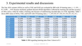
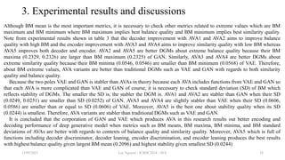
![3. Experimental results and discussions
As a result, let balance metric (BM) be the metric to assess quality of the generated image (the best image) with regard
to the ith image, which is formulated as follows:
BM𝑖 =
1
𝑛𝑖
𝑗
𝑑𝑖𝑗 1 − 𝑑𝑖𝑗
Where ni is the number of pixels of the ith image. The larger the BMi is, the better the generated image is, the better the
balance of similarity and diversity is. The overall BM of a DGM is average BM[i] over N=36 test images as follows:
BM =
1
𝑁
𝑖
BM𝑖 =
1
𝑁
𝑖
1
𝑛𝑖
𝑗
𝑑𝑖𝑗 1 − 𝑑𝑖𝑗 17
Where,
𝑑𝑖𝑗 = imageGen 𝑗 − image 𝑖 𝑗
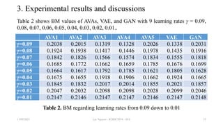
Recall that the larger the BM is, the better the DGM is. However, if the similarity quality is concern, the DGM will be
better when its BM is smaller because a small BM implies good similarity in this test with note that such small BM
implies small distance or small diversity. Therefore, the DGM whose BM is largest or smallest is preeminent. If the
DGM whose BM is largest, it is best in balance of similarity and diversity. If the DGM whose BM is smallest, it is best
in similarity. Both maximum and minimum of BM, which indicates both balance quality and similarity quality,
respectively, are concerned in this test but balance quality with large is more important.
13/09/2023 Loc Nguyen - ICBDC2024 - AVA 23](https://image.slidesharecdn.com/ava-icbdc2024-240601111212-b6aa6e1d/85/Adversarial-Variational-Autoencoders-to-extend-and-improve-generative-model-ICBDC2024-23-320.jpg)


The document discusses the development of Adversarial Variational Autoencoders (AVA), a unified model combining Variational Autoencoders (VAE) and Generative Adversarial Networks (GAN) to enhance generative AI capabilities. It highlights the strengths of both methods and presents a new architecture that integrates their functionalities, emphasizing the use of applied mathematics and programming techniques to improve data generation and reliability. The research methodology and theoretical foundations are outlined, aiming to demonstrate the effectiveness of AVA in generating accurate and realistic data.


![Polymer [ बहुलक ] Chemistry Notes PDF - Irfanullah Mehar - JJ Sir Chemistry.pdf](https://cdn.slidesharecdn.com/ss_thumbnails/polymerchemistrynotespdf-irfanullahmehar-jjsirchemistry-260210172118-3f9b37f7-thumbnail.jpg?width=640&height=640&fit=bounds)


