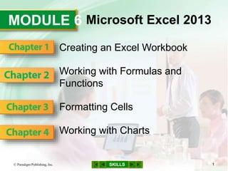
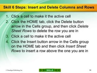
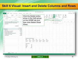
MODULE 6
SKILLS
Microsoft Excel 2013
Creating an Excel Workbook
Working with Formulas and
Functions
Formatting Cells
Working with Charts
© Paradigm Publishing, Inc. 1
SKILLS© Paradigm Publishing, Inc. 2
Creating an Excel Workbook
SKILLS
Guidelines to Planning and Creating a
Worksheet in Excel
© Paradigm Publishing, Inc. 3
SKILLS
Guidelines to Planning and Creating a
Worksheet in Excel…continued
© Paradigm Publishing, Inc. 4
 Take the time to plan how you will organize the
data on the worksheets
– consider the source data you will use and the results
you want to produce
– let your plan guide you as you enter the data
 If you want users to enter values in a
worksheet, position the input cells prominently
SKILLS
Guidelines to Planning and Creating a
Worksheet in Excel…continued
© Paradigm Publishing, Inc. 5
SKILLS
Guidelines to Planning and Creating a
Worksheet in Excel…continued
© Paradigm Publishing, Inc. 6
 You can use business logos, shapes, and other
graphics to enhance the appearance of your
worksheets
 Excel can also convey your worksheet data
graphically in a chart
 Charted data helps you spot trends and
abnormalities, which can help you make better
business decisions
 When planning a worksheet, keep in mind your
audience’s expectations as well as industry
standards
SKILLS
Skills You Learn
1. Understand worksheet and workbook structure
2. Use cell references
3. Enter text, values, and dates
4. Use the Auto Fill feature
5. Use the spelling checker
6. Insert and delete columns and rows
7. Work with multiple worksheets
8. Name and rename worksheets
9. Explore options for printing
© Paradigm Publishing, Inc. 7
SKILLS
Skill 1: Understand Worksheet
and Workbook Structure
© Paradigm Publishing, Inc. 8
SKILLS
Skill 1: Understand Worksheet
and Workbook Structure…continued
 Excel files are called workbooks
– a blank workbook contains one worksheet
– the capital letters across the top of the worksheet
are column headings
– the numbers down the left side are row headings
– the intersection of each row and column is a cell,
into which you can type an entry
– as you work, a heavy black border appears around
the active cell
© Paradigm Publishing, Inc. 9
SKILLS
Skill 1 Steps: Understand Worksheet
and Workbook Structure
1. Move the mouse pointer over the Formula bar
2. Click the New sheet button to add a worksheet
to the workbook and make it the active sheet
3. Click the Sheet1 tab to make it the active sheet
4. Click in a cell to make it the active cell
© Paradigm Publishing, Inc. 10
SKILLS
Skill 1 Steps…continued
5. Click the down arrow on the vertical scroll bar
to move down on the sheet
6. Click in cell A1 to make it the active cell
7. Press the Down Arrow key to move the cursor
to a different cell and make that cell active
8. Press and hold down the Shift key and then
press the Down Arrow key and the Right Arrow
to select a range
9. Click the Save button on the Quick Access
toolbar to save the file
© Paradigm Publishing, Inc. 11
SKILLS
Skill 1 Visual: Understand Worksheet and
Workbook Structure
© Paradigm Publishing, Inc. 12
Down arrow button on
the vertical scroll bar
Press the arrow keys to
move to a cell, or click in a
cell, to make it the active
cell.
Up arrow button on
the vertical scroll bar
SKILLS© Paradigm Publishing, Inc. 13
Jumping to a Cell
 You can jump directly to a cell by using the Go
To dialog box
 Open the Go To dialog box using one of these
methods:
– press F5
or
– click the Find & Select button in the Editing group on
the HOME tab and then click Go To
 In the Go To dialog box, enter a cell address in
the Reference text box and then click OK to
jump to that cell
CHECKPOINT QUESTION
SKILLS© Paradigm Publishing, Inc. 14
The capital letters across the top of the
worksheet are called
a. column headings
b. row headings
c. cell
d. active cell
1

SKILLS
Skill 2 Steps: Use Cell References
1. Type your name in cell A1 and press Enter
2. Click in a different cell to make it the active cell
3. Type =A1 and press Ctrl + Enter
4. Click in the Name box to the left of the Formula
bar
5. Type a cell address or a range (e.g., E5:G7)
and press Enter
© Paradigm Publishing, Inc. 15
SKILLS
Skill 2 Visual: Use Cell References
© Paradigm Publishing, Inc. 16
Look in the Formula bar and
verify that it displays the
entry you made, while the
cell itself displays the result.
SKILLS© Paradigm Publishing, Inc. 17
Making a Quick Analysis
 When you select a range of cells that contain
data, the Quick Analysis button appears at the
bottom right of the selected range
 Click the Quick Analysis button to display a
gallery where you can select from a variety of
tabs to analyze your data. For example:
– the CHARTS tab lets you display the selected data in
a chart
– the FORMATTING tab offers options that can be used
to quickly determine high and low values or highlight
values greater than a specified value
SKILLS© Paradigm Publishing, Inc. 18
Exploring a Worksheet
 A worksheet contains a fixed number of
columns and rows
 The number of usable cells depends upon the
amount of RAM available to your computer
 Cells within a worksheet can contain numbers
and dates in various formats, text, or formulas
using arithmetic operators or functions
– press End + Right Arrow to see the number of
columns in your worksheet
– press End + Down Arrow to see the number of rows in
your worksheet
CHECKPOINT QUESTION
SKILLS© Paradigm Publishing, Inc. 19
The column letter and row number make up
the cell reference or
a. value
b. range name
c. cell address
d. formula
2

SKILLS
Skill 3 Steps: Enter Text, Values, and Dates
1. Make cell A1 the active cell, type Chocolate
and the Aztec Culture Exhibit, and then press
Enter
2. Type Exhibit Plan in cell A2 and then press
Enter twice
3. Type 3-26-15 in cell A4 and then press Enter
4. Make cell B6 the active cell, type Due Date,
and then press Enter
5. Make cell A7 the active cell and type the
remaining entries into the range A7:A13
© Paradigm Publishing, Inc. 20
SKILLS
Skill 3 Steps…continued
6. Make cell B7 the active cell and type the
remaining entries into the range B7:B13
7. Move the mouse pointer over the divider line
between the column A and column B headings
until it turns into a left-and-right-pointing arrow
8. Double-click the divider line between the
column A and column B headings to resize
column A
© Paradigm Publishing, Inc. 21
SKILLS
Skill 3 Visual: Enter Text, Values, and Dates
© Paradigm Publishing, Inc. 22
Excel automatically
reformats the date.
SKILLS© Paradigm Publishing, Inc. 23
Removing ### from a Cell
 In certain situations, such as when you enter a
very large number in a cell, Excel displays a
series of pound signs (###) rather than the
entry itself
 These signs indicate that the numeric entry is
too wide to display in the cell
 Increase the column width for the cell contents
to display properly
CHECKPOINT QUESTION
SKILLS© Paradigm Publishing, Inc. 24
If a date is typed as 4-27-15, Excel will
display the date as
a. 4-27-15
b. 4-27-2015
c. 4/27/15
d. 4/27/2015
3

SKILLS
Skill 4 Steps: Use the Auto Fill Feature
1. Click in a cell to make it the active cell, type Mon,
and press Ctrl + Enter
2. Move the mouse pointer over the fill handle in
the lower right corner of the cell, press and hold
down the left mouse button, and then drag to the
right until you see a ScreenTip that reads Sun
3. Release the mouse button
© Paradigm Publishing, Inc. 25
SKILLS
Skill 4 Steps…continued
4. Make a cell the active cell, type 10 a.m., and
then press Enter
5. Drag over a range that begins with 10 a.m.,
click the Fill button in the Editing group on the
HOME tab, and then click the Right option
6. Make a cell the active cell, type $4, press Enter,
type $6, and then press Enter
7. Drag over the two typed dollar amounts
8. Drag the fill handle down to finish filling the
custom series to $10 and then release the left
mouse button
© Paradigm Publishing, Inc. 26
SKILLS
Skill 4 Visual: Use the Auto Fill Feature
© Paradigm Publishing, Inc. 27
Drag the fill handle
down to finish filling
the custom series to
$10 and then release
the mouse button.
SKILLS© Paradigm Publishing, Inc. 28
Using Flash Fill
 Flash Fill will save you time when entering data
that is repeated in a pattern
 Here is an example:
– suppose you enter a list of employee email addresses
in column A, and each email address contains the
employee’s last name and first initial
– when you start typing employee last names in
column B, Excel will recognize the pattern and fill in
the remaining last names in column B
CHECKPOINT QUESTION
SKILLS© Paradigm Publishing, Inc. 29
The _____ feature enables you to create a
series of entries down a column or across a
row.
a. Copy
b. Auto Fill
c. Templates
d. Clear
4

SKILLS
Skill 5 Steps: Use the Spelling Checker
1. Make cell A1 the active cell
2. Click the REVIEW tab and then click the
Spelling button in the Proofing group to open
the Spelling dialog box with the first mistake
displayed
3. Click the Change button to replace the
misspelled word with the correct spelling that is
selected in the Suggestions list box
4. Continue clicking the Change button to correct
the remaining misspellings and click OK in the
message box
© Paradigm Publishing, Inc. 30
SKILLS
Skill 5 Visual: Use the Spelling Checker
© Paradigm Publishing, Inc. 31
Click the Change button to
replace the misspelled
word with the correct
spelling that is selected in
the Suggestions list box.
SKILLS© Paradigm Publishing, Inc. 32
Using Auto Correct
 You can customize the AutoCorrect feature so
that a correction will be made:
1. click the FILE tab and then click Options
2. click Proofing at the left side of the Excel Options
dialog box and then click the AutoCorrect Options
button in the right panel
3. in the AutoCorrect dialog box, with the AutoCorrect
tab selected, type your frequent typo (such as
Simth) in the Replace text box and then type the
correction (Smith in this instance) in the With text
box
4. click Add and then click OK twice
CHECKPOINT QUESTION
SKILLS© Paradigm Publishing, Inc. 33
The spelling checker can find errors in these
types of entries.
a. text
b. values
c. dates
d. worksheet names
5

SKILLS
Skill 6 Steps: Insert and Delete Columns and Rows
1. Click a cell to make it the active cell
2. Click the HOME tab, click the Delete button
arrow in the Cells group, and then click Delete
Sheet Rows to delete the row you are in
3. Click a cell to make it the active cell
4. Click the Insert button arrow in the Cells group
on the HOME tab and then click Insert Sheet
Rows to insert a row above the one you are in
© Paradigm Publishing, Inc. 34
SKILLS
Skill 6 Visual: Insert and Delete Columns and Rows
© Paradigm Publishing, Inc. 35
Click the Delete button
arrow in the Cells group
on the HOME tab and
then click Delete Sheet
Rows.
SKILLS© Paradigm Publishing, Inc. 36
Designing Worksheets Using Rows and
Columns
 Rows and columns can play both functional and
design roles in your worksheet
 For example:
– when you perform calculations and certain other
activities such as charting, you will find the actions
easiest to perform when all the data is located in
adjoining rows and columns
CHECKPOINT QUESTION
SKILLS© Paradigm Publishing, Inc. 37
Doing this to a row or column removes it and
its contents.
a. inserting
b. copying
c. deleting
d. summing
6

SKILLS
Skill 7 Steps: Work with Multiple Worksheets
Delete Multiple Worksheets
1. Click the New sheet button to add Sheet3
2. Click the Sheet2 tab, press and hold down the
Ctrl key, and then click the Sheet3 tab to select
Sheet2 and Sheet3
3. In the Cells group on the HOME tab, click the
Delete button arrow
4. Click Delete Sheet
5. Click the Delete button in the message box
warning you that sheets may contain data that
will be deleted
© Paradigm Publishing, Inc. 38
SKILLS
Skill 7 Steps…continued
Copy a Worksheet
1. Right-click the Sheet1 sheet tab and then click
Move or Copy
2. Click (move to end) in the Before sheet list box
in the Move or Copy dialog box
3. Click the Create a copy check box to insert a
check mark
4. Click OK
© Paradigm Publishing, Inc. 39
SKILLS
Skill 7 Visual: Work with Multiple Worksheets
© Paradigm Publishing, Inc. 40
Right-click a sheet tab
and then click Move or
Copy to open the Move
or Copy dialog box.
SKILLS© Paradigm Publishing, Inc. 41
Copying Data to Another Workbook
 You may have noticed that the Move or Copy
dialog box includes a To book option box
 If you have another workbook open, you can
select it in this option box to move or copy the
specified worksheet to that workbook
CHECKPOINT QUESTION
SKILLS© Paradigm Publishing, Inc. 42
This key allows you to select multiple items,
including multiple worksheet tabs.
a. Alt
b. Shift
c. Esc
d. Ctrl
7

SKILLS
Skill 8 Steps: Name and Rename Worksheets
1. Right-click a sheet tab
2. Click Rename
3. Type a sheet name and press Enter
© Paradigm Publishing, Inc. 43
SKILLS
Skill 8 Visual: Name and Rename Worksheets
© Paradigm Publishing, Inc. 44
Right-click a sheet tab
and then click the
Rename option in the
shortcut menu.
SKILLS© Paradigm Publishing, Inc. 45
Color Coding Sheet Tabs
 Color-coding worksheet tabs is another way to
make it easier to find data in a workbook
 To change the color of a sheet tab:
1. right-click the tab
2. point to Tab Color
3. click the color you want from the palette
CHECKPOINT QUESTION
SKILLS© Paradigm Publishing, Inc. 46
Change the _____ for a worksheet on the
sheet tab to describe its contents.
a. theme
b. color
c. value
d. name
8

SKILLS
Skill 9 Steps: Explore Options for Printing
1. Click the FILE tab
2. Click the Print option to open the Print
backstage area, which displays print settings
and a preview of the printout
3. Click the Print button
© Paradigm Publishing, Inc. 47
SKILLS
Skill 9 Visual: Explore Options for Printing
© Paradigm Publishing, Inc. 48
A preview of the printout
displays in the Print
backstage area.
SKILLS© Paradigm Publishing, Inc. 49
Adding Headers and Footers
 Headers and footers can include identifying
information such as the file name, your name,
your company name, or page numbers
 To add a header or a footer:
1. click the INSERT tab and then click the Header &
Footer button in the Text group
2. type information in the placeholders that appear on
the worksheet for the header or footer
3. use the choices on the HEADER & FOOTER
TOOLS DESIGN tab to insert elements such as
page numbers and the file name
CHECKPOINT QUESTION
SKILLS© Paradigm Publishing, Inc. 50
Click the Print button on the FILE tab to
display printing choices in the
a. Print backstage area
b. Print Preview view
c. Print dialog box
d. PAGE LAYOUT tab
9

SKILLS
Tasks Summary: 1 of 2
© Paradigm Publishing, Inc. 51
SKILLS
Tasks Summary: 2 of 2
© Paradigm Publishing, Inc. 52

Gl13 m6-c1-presentation

  • 1.
    MODULE 6 SKILLS Microsoft Excel2013 Creating an Excel Workbook Working with Formulas and Functions Formatting Cells Working with Charts © Paradigm Publishing, Inc. 1
  • 2.
    SKILLS© Paradigm Publishing,Inc. 2 Creating an Excel Workbook
  • 3.
    SKILLS Guidelines to Planningand Creating a Worksheet in Excel © Paradigm Publishing, Inc. 3
  • 4.
    SKILLS Guidelines to Planningand Creating a Worksheet in Excel…continued © Paradigm Publishing, Inc. 4  Take the time to plan how you will organize the data on the worksheets – consider the source data you will use and the results you want to produce – let your plan guide you as you enter the data  If you want users to enter values in a worksheet, position the input cells prominently
  • 5.
    SKILLS Guidelines to Planningand Creating a Worksheet in Excel…continued © Paradigm Publishing, Inc. 5
  • 6.
    SKILLS Guidelines to Planningand Creating a Worksheet in Excel…continued © Paradigm Publishing, Inc. 6  You can use business logos, shapes, and other graphics to enhance the appearance of your worksheets  Excel can also convey your worksheet data graphically in a chart  Charted data helps you spot trends and abnormalities, which can help you make better business decisions  When planning a worksheet, keep in mind your audience’s expectations as well as industry standards
  • 7.
    SKILLS Skills You Learn 1.Understand worksheet and workbook structure 2. Use cell references 3. Enter text, values, and dates 4. Use the Auto Fill feature 5. Use the spelling checker 6. Insert and delete columns and rows 7. Work with multiple worksheets 8. Name and rename worksheets 9. Explore options for printing © Paradigm Publishing, Inc. 7
  • 8.
    SKILLS Skill 1: UnderstandWorksheet and Workbook Structure © Paradigm Publishing, Inc. 8
  • 9.
    SKILLS Skill 1: UnderstandWorksheet and Workbook Structure…continued  Excel files are called workbooks – a blank workbook contains one worksheet – the capital letters across the top of the worksheet are column headings – the numbers down the left side are row headings – the intersection of each row and column is a cell, into which you can type an entry – as you work, a heavy black border appears around the active cell © Paradigm Publishing, Inc. 9
  • 10.
    SKILLS Skill 1 Steps:Understand Worksheet and Workbook Structure 1. Move the mouse pointer over the Formula bar 2. Click the New sheet button to add a worksheet to the workbook and make it the active sheet 3. Click the Sheet1 tab to make it the active sheet 4. Click in a cell to make it the active cell © Paradigm Publishing, Inc. 10
  • 11.
    SKILLS Skill 1 Steps…continued 5.Click the down arrow on the vertical scroll bar to move down on the sheet 6. Click in cell A1 to make it the active cell 7. Press the Down Arrow key to move the cursor to a different cell and make that cell active 8. Press and hold down the Shift key and then press the Down Arrow key and the Right Arrow to select a range 9. Click the Save button on the Quick Access toolbar to save the file © Paradigm Publishing, Inc. 11
  • 12.
    SKILLS Skill 1 Visual:Understand Worksheet and Workbook Structure © Paradigm Publishing, Inc. 12 Down arrow button on the vertical scroll bar Press the arrow keys to move to a cell, or click in a cell, to make it the active cell. Up arrow button on the vertical scroll bar
  • 13.
    SKILLS© Paradigm Publishing,Inc. 13 Jumping to a Cell  You can jump directly to a cell by using the Go To dialog box  Open the Go To dialog box using one of these methods: – press F5 or – click the Find & Select button in the Editing group on the HOME tab and then click Go To  In the Go To dialog box, enter a cell address in the Reference text box and then click OK to jump to that cell
  • 14.
    CHECKPOINT QUESTION SKILLS© ParadigmPublishing, Inc. 14 The capital letters across the top of the worksheet are called a. column headings b. row headings c. cell d. active cell 1 
  • 15.
    SKILLS Skill 2 Steps:Use Cell References 1. Type your name in cell A1 and press Enter 2. Click in a different cell to make it the active cell 3. Type =A1 and press Ctrl + Enter 4. Click in the Name box to the left of the Formula bar 5. Type a cell address or a range (e.g., E5:G7) and press Enter © Paradigm Publishing, Inc. 15
  • 16.
    SKILLS Skill 2 Visual:Use Cell References © Paradigm Publishing, Inc. 16 Look in the Formula bar and verify that it displays the entry you made, while the cell itself displays the result.
  • 17.
    SKILLS© Paradigm Publishing,Inc. 17 Making a Quick Analysis  When you select a range of cells that contain data, the Quick Analysis button appears at the bottom right of the selected range  Click the Quick Analysis button to display a gallery where you can select from a variety of tabs to analyze your data. For example: – the CHARTS tab lets you display the selected data in a chart – the FORMATTING tab offers options that can be used to quickly determine high and low values or highlight values greater than a specified value
  • 18.
    SKILLS© Paradigm Publishing,Inc. 18 Exploring a Worksheet  A worksheet contains a fixed number of columns and rows  The number of usable cells depends upon the amount of RAM available to your computer  Cells within a worksheet can contain numbers and dates in various formats, text, or formulas using arithmetic operators or functions – press End + Right Arrow to see the number of columns in your worksheet – press End + Down Arrow to see the number of rows in your worksheet
  • 19.
    CHECKPOINT QUESTION SKILLS© ParadigmPublishing, Inc. 19 The column letter and row number make up the cell reference or a. value b. range name c. cell address d. formula 2 
  • 20.
    SKILLS Skill 3 Steps:Enter Text, Values, and Dates 1. Make cell A1 the active cell, type Chocolate and the Aztec Culture Exhibit, and then press Enter 2. Type Exhibit Plan in cell A2 and then press Enter twice 3. Type 3-26-15 in cell A4 and then press Enter 4. Make cell B6 the active cell, type Due Date, and then press Enter 5. Make cell A7 the active cell and type the remaining entries into the range A7:A13 © Paradigm Publishing, Inc. 20
  • 21.
    SKILLS Skill 3 Steps…continued 6.Make cell B7 the active cell and type the remaining entries into the range B7:B13 7. Move the mouse pointer over the divider line between the column A and column B headings until it turns into a left-and-right-pointing arrow 8. Double-click the divider line between the column A and column B headings to resize column A © Paradigm Publishing, Inc. 21
  • 22.
    SKILLS Skill 3 Visual:Enter Text, Values, and Dates © Paradigm Publishing, Inc. 22 Excel automatically reformats the date.
  • 23.
    SKILLS© Paradigm Publishing,Inc. 23 Removing ### from a Cell  In certain situations, such as when you enter a very large number in a cell, Excel displays a series of pound signs (###) rather than the entry itself  These signs indicate that the numeric entry is too wide to display in the cell  Increase the column width for the cell contents to display properly
  • 24.
    CHECKPOINT QUESTION SKILLS© ParadigmPublishing, Inc. 24 If a date is typed as 4-27-15, Excel will display the date as a. 4-27-15 b. 4-27-2015 c. 4/27/15 d. 4/27/2015 3 
  • 25.
    SKILLS Skill 4 Steps:Use the Auto Fill Feature 1. Click in a cell to make it the active cell, type Mon, and press Ctrl + Enter 2. Move the mouse pointer over the fill handle in the lower right corner of the cell, press and hold down the left mouse button, and then drag to the right until you see a ScreenTip that reads Sun 3. Release the mouse button © Paradigm Publishing, Inc. 25
  • 26.
    SKILLS Skill 4 Steps…continued 4.Make a cell the active cell, type 10 a.m., and then press Enter 5. Drag over a range that begins with 10 a.m., click the Fill button in the Editing group on the HOME tab, and then click the Right option 6. Make a cell the active cell, type $4, press Enter, type $6, and then press Enter 7. Drag over the two typed dollar amounts 8. Drag the fill handle down to finish filling the custom series to $10 and then release the left mouse button © Paradigm Publishing, Inc. 26
  • 27.
    SKILLS Skill 4 Visual:Use the Auto Fill Feature © Paradigm Publishing, Inc. 27 Drag the fill handle down to finish filling the custom series to $10 and then release the mouse button.
  • 28.
    SKILLS© Paradigm Publishing,Inc. 28 Using Flash Fill  Flash Fill will save you time when entering data that is repeated in a pattern  Here is an example: – suppose you enter a list of employee email addresses in column A, and each email address contains the employee’s last name and first initial – when you start typing employee last names in column B, Excel will recognize the pattern and fill in the remaining last names in column B
  • 29.
    CHECKPOINT QUESTION SKILLS© ParadigmPublishing, Inc. 29 The _____ feature enables you to create a series of entries down a column or across a row. a. Copy b. Auto Fill c. Templates d. Clear 4 
  • 30.
    SKILLS Skill 5 Steps:Use the Spelling Checker 1. Make cell A1 the active cell 2. Click the REVIEW tab and then click the Spelling button in the Proofing group to open the Spelling dialog box with the first mistake displayed 3. Click the Change button to replace the misspelled word with the correct spelling that is selected in the Suggestions list box 4. Continue clicking the Change button to correct the remaining misspellings and click OK in the message box © Paradigm Publishing, Inc. 30
  • 31.
    SKILLS Skill 5 Visual:Use the Spelling Checker © Paradigm Publishing, Inc. 31 Click the Change button to replace the misspelled word with the correct spelling that is selected in the Suggestions list box.
  • 32.
    SKILLS© Paradigm Publishing,Inc. 32 Using Auto Correct  You can customize the AutoCorrect feature so that a correction will be made: 1. click the FILE tab and then click Options 2. click Proofing at the left side of the Excel Options dialog box and then click the AutoCorrect Options button in the right panel 3. in the AutoCorrect dialog box, with the AutoCorrect tab selected, type your frequent typo (such as Simth) in the Replace text box and then type the correction (Smith in this instance) in the With text box 4. click Add and then click OK twice
  • 33.
    CHECKPOINT QUESTION SKILLS© ParadigmPublishing, Inc. 33 The spelling checker can find errors in these types of entries. a. text b. values c. dates d. worksheet names 5 
  • 34.
    SKILLS Skill 6 Steps:Insert and Delete Columns and Rows 1. Click a cell to make it the active cell 2. Click the HOME tab, click the Delete button arrow in the Cells group, and then click Delete Sheet Rows to delete the row you are in 3. Click a cell to make it the active cell 4. Click the Insert button arrow in the Cells group on the HOME tab and then click Insert Sheet Rows to insert a row above the one you are in © Paradigm Publishing, Inc. 34
  • 35.
    SKILLS Skill 6 Visual:Insert and Delete Columns and Rows © Paradigm Publishing, Inc. 35 Click the Delete button arrow in the Cells group on the HOME tab and then click Delete Sheet Rows.
  • 36.
    SKILLS© Paradigm Publishing,Inc. 36 Designing Worksheets Using Rows and Columns  Rows and columns can play both functional and design roles in your worksheet  For example: – when you perform calculations and certain other activities such as charting, you will find the actions easiest to perform when all the data is located in adjoining rows and columns
  • 37.
    CHECKPOINT QUESTION SKILLS© ParadigmPublishing, Inc. 37 Doing this to a row or column removes it and its contents. a. inserting b. copying c. deleting d. summing 6 
  • 38.
    SKILLS Skill 7 Steps:Work with Multiple Worksheets Delete Multiple Worksheets 1. Click the New sheet button to add Sheet3 2. Click the Sheet2 tab, press and hold down the Ctrl key, and then click the Sheet3 tab to select Sheet2 and Sheet3 3. In the Cells group on the HOME tab, click the Delete button arrow 4. Click Delete Sheet 5. Click the Delete button in the message box warning you that sheets may contain data that will be deleted © Paradigm Publishing, Inc. 38
  • 39.
    SKILLS Skill 7 Steps…continued Copya Worksheet 1. Right-click the Sheet1 sheet tab and then click Move or Copy 2. Click (move to end) in the Before sheet list box in the Move or Copy dialog box 3. Click the Create a copy check box to insert a check mark 4. Click OK © Paradigm Publishing, Inc. 39
  • 40.
    SKILLS Skill 7 Visual:Work with Multiple Worksheets © Paradigm Publishing, Inc. 40 Right-click a sheet tab and then click Move or Copy to open the Move or Copy dialog box.
  • 41.
    SKILLS© Paradigm Publishing,Inc. 41 Copying Data to Another Workbook  You may have noticed that the Move or Copy dialog box includes a To book option box  If you have another workbook open, you can select it in this option box to move or copy the specified worksheet to that workbook
  • 42.
    CHECKPOINT QUESTION SKILLS© ParadigmPublishing, Inc. 42 This key allows you to select multiple items, including multiple worksheet tabs. a. Alt b. Shift c. Esc d. Ctrl 7 
  • 43.
    SKILLS Skill 8 Steps:Name and Rename Worksheets 1. Right-click a sheet tab 2. Click Rename 3. Type a sheet name and press Enter © Paradigm Publishing, Inc. 43
  • 44.
    SKILLS Skill 8 Visual:Name and Rename Worksheets © Paradigm Publishing, Inc. 44 Right-click a sheet tab and then click the Rename option in the shortcut menu.
  • 45.
    SKILLS© Paradigm Publishing,Inc. 45 Color Coding Sheet Tabs  Color-coding worksheet tabs is another way to make it easier to find data in a workbook  To change the color of a sheet tab: 1. right-click the tab 2. point to Tab Color 3. click the color you want from the palette
  • 46.
    CHECKPOINT QUESTION SKILLS© ParadigmPublishing, Inc. 46 Change the _____ for a worksheet on the sheet tab to describe its contents. a. theme b. color c. value d. name 8 
  • 47.
    SKILLS Skill 9 Steps:Explore Options for Printing 1. Click the FILE tab 2. Click the Print option to open the Print backstage area, which displays print settings and a preview of the printout 3. Click the Print button © Paradigm Publishing, Inc. 47
  • 48.
    SKILLS Skill 9 Visual:Explore Options for Printing © Paradigm Publishing, Inc. 48 A preview of the printout displays in the Print backstage area.
  • 49.
    SKILLS© Paradigm Publishing,Inc. 49 Adding Headers and Footers  Headers and footers can include identifying information such as the file name, your name, your company name, or page numbers  To add a header or a footer: 1. click the INSERT tab and then click the Header & Footer button in the Text group 2. type information in the placeholders that appear on the worksheet for the header or footer 3. use the choices on the HEADER & FOOTER TOOLS DESIGN tab to insert elements such as page numbers and the file name
  • 50.
    CHECKPOINT QUESTION SKILLS© ParadigmPublishing, Inc. 50 Click the Print button on the FILE tab to display printing choices in the a. Print backstage area b. Print Preview view c. Print dialog box d. PAGE LAYOUT tab 9 
  • 51.
    SKILLS Tasks Summary: 1of 2 © Paradigm Publishing, Inc. 51
  • 52.
    SKILLS Tasks Summary: 2of 2 © Paradigm Publishing, Inc. 52

Editor's Notes

  • #2 In Module 6, you learn about Microsoft Excel 2013. Chapter 1 covers creating an Excel workbook, including entering data and navigating. Chapter 2 deals with performing calculations. In Chapter 3, you use formatting tools to add visual appeal. In Chapter 4, you learn about working with charts and graphs.
  • #3 You are continuing your work for The Chocolate Museum, a nonprofit organization that provides educational exhibits and information on the history of chocolate and its role in world cultures. The Museum must plan and budget for its exhibits and gift shop, and this planning requires tracking dates and calculating financial information. In this chapter, you produce an Excel workbook containing schedule and cost information for a new exhibit on chocolate in world cultures.
  • #4 The data should guide your decisions about the best way to lay out a workbook and organize data on the worksheets.
  • #5 Once you have entered and organized data on the worksheets, you can make any necessary calculations. For example, if you have four columns of quarterly sales data, you can create a formula that sums the values of each column to give you a quarterly total. And for each data row, you can create a formula that sums the results for the product in each row. If your worksheet includes an area where the user enters values to be calculated by Excel, position those input cells in a prominent location—usually near the top of the worksheet or on a separate worksheet—and apply formatting that prompts the user for entries
  • #6 Charts convey data graphically, allowing you to easily spot trends and abnormalities.
  • #7 Examples Charted data can help you quickly identify the trend if sales for a particular product lag far behind sales for other products. You need to keep industry standards in mind in the financial industry, where professionals follow accepted conventions and, in some cases, legal requirements when they design reports such as profit and loss statements, balance sheets, and loan payment tables.
  • #8 In this chapter, you learn how to enter data and navigate in Excel. Because you will be dealing with different types of data—numbers, text, and dates—you will learn how to enter each type of data to ensure that your calculations work. There are tools and tricks to help you out, such as automatically filling entries, quickly adding rows or columns, or checking the spelling of cell contents. Rather than setting up each Excel spreadsheet as a single and lengthy page of data, you learn how to organize data on multiple pages, called worksheets, to help you group like kinds of data on their own sheets and make navigating your data easier. If you have sales data for different years, for example, you can track each year’s data on a separate sheet in a single workbook. You can add sheets to a workbook and name and rename sheets as needed so that the data is easy to find and work with. Finally, you will learn how to set up and print a worksheet. Navigation Tip: In Slide Show view, click an underlined skill on this slide to navigate directly to the related slide. At any time in Slide Show view, you may navigate to the beginning of this presentation by clicking the left-most button at the bottom center of the slide. To navigate to the previous slide in this presentation, click the second button from the left. Click the SKILLS button to return to this slide. Click the button to the right of the SKILLS button to navigate to the next slide in this presentation, and click the right-most button to navigate to the end of this presentation.
  • #9 Workbooks are like notebooks. Worksheets are like pages in a notebook. You can add worksheets, or sheets, to your workbook to keep your data organized. Column headings identify each column. Row headings identify each row. You can only make entries in the active cell. You can use the Formula bar located above the column headings to view and work with the entered data and modify individual cells or a range of cells.
  • #10 When you start Excel, you can create a blank workbook or select a workbook template. An entry can be a data value like a name, number, or date, or a formula that instructs Excel to perform a calculation.
  • #11 To open Excel, click the Excel 2013 tile on the Start screen or press Win + C , click the Search charm, and then type Excel. A ScreenTip that reads Formula Bar appears to identify that screen element. Only one sheet can be active at any given time. The active sheet is shown with its name underlined in its tab. The active cell is highlighted with a black border, and the cell name appears in the Name box next to the Formula bar.
  • #12 Click the up arrow on the vertical scroll bar to move up on the sheet. The shortcut to make A1 the active cell is Ctrl + Home. You can also use the Up Arrow, Right Arrow, and Left Arrow keys to move the cursor to a different cell and make that cell active. You can use the Shift key and any combination of the Down Arrow, Up Arrow, Right Arrow, and Left Arrow to select a range. Another Way: Use the Click, Shift-Click method to select a range: press the left mouse button and drag over the range or click the upper left cell and hold down Shift as you click the lower right cell.
  • #13 Click the down arrow and up arrow buttons on the vertical scroll bar, as shown in the illustration in this slide, to move down or up the page. Notice that scrolling does not change the selected cell.
  • #14 The Go To dialog box is another way to move to a cell and make it the active cell.
  • #15 Navigation Tip: In Slide Show view, read the Checkpoint question and determine which answer is the correct answer. Click anywhere on the slide, and the correct answer will display in green with a green check mark beside it.
  • #16 You can identify each cell by its column letter and row number, called its cell address, cell reference, or cell name. The entire content of a data cell will display even if it is too long to fit in the cell as long as the cell immediately to the right is empty. If the cell immediately to the right contains data, the overflow cell content will be hidden. The entire contents of a cell will always display in the Formula bar. All Excel formulas begin with an equals sign. When you type a formula in Excel, you may enter letters as either capital or lowercase. The program automatically capitalizes the letters in the cell as you type. Pressing Ctrl + Enter finishes entering the formula and keeps the cell active. You can use the Name box to the left of the Formula bar to go to a cell or range. When you type a range in the Name box, the range of cells is selected. Identify a range by the addresses of its upper left and lower right cells, separating the addresses with a colon. A range can span multiple rows and columns, as it does in the example given in the slide (E5:G7). Alternatively, it can span a single row, as in A3:F3. A range also can fall within a single column, as in C3:C10.
  • #17 The illustration in this slide shows a formula entered in the active cell, F6, that references the contents in cell A1. Understanding cell and range addresses is also important when building formulas, a skill you will learn about in Module 6, Chapter 2.
  • #18 The Quick Analysis button provides hand access to a variety of ways to analyze your data.
  • #19 A worksheet contains numerous columns and rows. Columns are lettered A–Z and then continue in an AA, AB, AC ... BA, BB, BC format. Rows are numbered sequentially.
  • #20 Navigation Tip: In Slide Show view, read the Checkpoint question and determine which answer is the correct answer. Click anywhere on the slide, and the correct answer will display in green with a green check mark beside it.
  • #21 Each cell in an Excel worksheet can hold a single entry. That entry can be text, a date, a value, or a formula that calculates a result. A text entry can contain any combination of letters, numbers, or symbols that you can type on your keyboard. Qtr 1, Sales, or Region# are examples of text entries. By default, Excel aligns text entries at the left side of the cell. This is true even of phone numbers because they usually are entered with hyphens or other characters and are treated as text. Numbers are numeric entries, including whole numbers (15) and decimal values (2.5). You can enter numbers that have certain characteristics, such as currency symbols or a number of decimal places. Number entries are right-aligned. Another Way: Press the Down Arrow key to finish a cell entry and move one cell down, the Right or Left Arrow keys to move one column to the right or left, or the Up Arrow key to move up one row. You enter dates in typical date formats, with hyphens (4-1-15) or slashes (4/1/15). By default, if you enter 4/1/15 or 4-1-15, Excel displays 4/1/2015 in the cell.
  • #22 Notice that the date entries in column B appear to have cut off the entries in column A. The length of the entries requires that you resize column A to accommodate them. Click a cell and look at the Formula bar to confirm that the entire entry is retained in a cell even when it is only partially displayed. The length of the entries requires that you resize column A to accommodate them.
  • #23 The illustration in this slide displays two date formats. In cell A4, the date was typed as 3-26-15. In cell B7, the date was typed as 5/18. Notice how Excel automatically reformats the date.
  • #24 This feature (displaying pound signs) is designed to keep readers of the data from being mislead by seeing only a portion of a number. You will learn more about sizing cells in Chapter 3, Skill 3.
  • #25 Navigation Tip: In Slide Show view, read the Checkpoint question and determine which answer is the correct answer. Click anywhere on the slide, and the correct answer will display in green with a green check mark beside it.
  • #26 The Auto Fill and Flash Fill features in Excel 2013 can help you save time when entering data. Auto Fill enables you to either copy an entry across a row or down a column or create a series of entries across a row or down a column. For example, if you enter Jan in a cell and use the Auto Fill feature, Excel enters the following months: Feb, Mar, Apr, and so on. Ctrl + Enter finishes an entry without moving the cursor to another cell. The fill handle looks like a small square. Drag when the mouse pointer changes to a black crosshair. Click the Auto Fill Options button that appears after a fill if you want to change the fill. For example, you might want to fill formatting only or copy cells rather than fill a series.
  • #27 Auto Fill can also be used to fill the days of the week or common business entries such as Qtr 1, Qtr 2, and so on. If you use Auto Fill to enter a number or other entry that Excel does not recognize as part of a series, Excel simply copies the entry to the area you are filling. You can create your own series by entering the first two or three values in the series and then using Auto Fill from there. Excel copies the 10 a.m. entry across the selected range. Excel will not fill all times correctly. For example, it fills 12 p.m. and then 13 p.m., an obvious error. You can type some number formats, such as dollar signs and percent signs, when entering the numbers, or you can apply number formatting later.
  • #28 The illustration in this slide shows the two dollar amounts that you typed, $4 and $6, selected and the fill handle being dragged down to finish filling the custom series to $10.
  • #29 Flash Fill looks for patterns in your data and then automatically enters the rest of your data based on the pattern.
  • #30 Navigation Tip: In Slide Show view, read the Checkpoint question and determine which answer is the correct answer. Click anywhere on the slide, and the correct answer will display in green with a green check mark beside it.
  • #31 Spreadsheets can be filled with typos, requiring an eagle-eyed person to read closely to find and eliminate those pesky misspellings. Excel includes a feature to help you ensure that your worksheets are free of typos. The Excel spelling checker works much like the Word spelling checker, except that it opens in a dialog box instead of a pane. There is one extra caution with using this feature in Excel: the spelling checker only reviews text entries. It cannot ensure that you have entered numbers and dates correctly, so double-check your data thoroughly! The spelling checker starts from the current cell, and Excel displays a message when it needs to return to the beginning of the sheet. You can also turn on the spelling checker with the keyboard shortcut F7. The message box informs you that the spelling check is complete.
  • #32 In the illustration in this slide, the Spelling dialog box displays the first typing mistake, Recriut. The correct spelling is already selected in the Suggestions list box, so click the Change button to replace the misspelled word.
  • #33 Excel can correct some misspellings for you as you type. Each of us has our own unique tendency to mistype certain words. For example, perhaps your last name is Smith, but you often mistype it as Simth. Excel cannot, by default, correct that mistake. However, you can customize the AutoCorrect feature so that the correction will be made.
  • #34 Navigation Tip: In Slide Show view, read the Checkpoint question and determine which answer is the correct answer. Click anywhere on the slide, and the correct answer will display in green with a green check mark beside it.
  • #35 You can insert and delete rows and columns within your data to rearrange the data or make room for new data. For example, if you created a worksheet to track the value of products in your company’s inventory, you might need to add rows for new products that you add to your catalog or remove rows when products are discontinued. Each Excel worksheet always has the same number of rows and columns. When you insert and delete rows and columns, you are simply changing where the blank rows and columns appear in the sheet. Another Way: Right-click a column or row heading and use the Delete option. When you delete a row, Excel removes the row immediately and does not display a warning that you will be deleting the contents of the row. If you accidentally delete the wrong row or column, immediately click the Undo button on the Quick Access toolbar to restore the deleted content. Another Way: Right-click a column or row heading and use the Insert option.
  • #36 The illustration in this slide shows one method to delete a sheet row. Before deleting rows and columns, save your worksheet. Make sure to check the rows and columns before you delete them to be sure you will not be losing important data.
  • #38 Navigation Tip: In Slide Show view, read the Checkpoint question and determine which answer is the correct answer. Click anywhere on the slide, and the correct answer will display in green with a green check mark beside it.
  • #39 Given the size of each worksheet, it would be possible to arrange a wide variety of different sets of data in ranges spread throughout a single sheet. However, you would have to spend a lot of time scrolling and otherwise navigating to find the section of the sheet containing the data you want to view and use. Dividing data into multiple worksheets is often more efficient for reading the data. Each Excel workbook enables you to create multiple worksheets. If you have to track data for many stores, no problem! You can create a sheet for each one or copy an existing sheet to a new sheet for editing. You also can delete sheets with old data you no longer need. This skill offers instruction and practice for all of these options. The Ctrl key allows you to select multiple items, including multiple worksheet tabs. Another Way: You can right-click a sheet tab and then click Delete at the shortcut menu. The new sheet, named Sheet1 (2), appears and is the active sheet.
  • #40 The new sheet, named Sheet1 (2), appears and is the active sheet.
  • #41 The illustration in this slide displays the Move or Copy dialog box that opens when you right-click a sheet tab and click the Move or Copy option.
  • #42 This action enables you to transfer data to other workbook files using a method that is faster than copying and pasting.
  • #43 Navigation Tip: In Slide Show view, read the Checkpoint question and determine which answer is the correct answer. Click anywhere on the slide, and the correct answer will display in green with a green check mark beside it.
  • #44 If the goal of adding worksheets is to make information easier to find and identify, then “mystery” worksheet names, such as Sheet1 and Sheet2, certainly do not help. Giving each worksheet a unique name that identifies its contents makes it much easier to determine which tab to click to find the data you need. Use the worksheet tab to rename the worksheet. You could also double-click the Sheet tab, type the sheet name, and then press Enter.
  • #45 The illustration in this slide shows the shortcut menu that displays if you right-click a sheet tab. A sheet name can be up to 31 characters and can contain most characters on the keyboard, including spaces. Only a handful of characters, such as / (slash), (backslash), * (asterisk), ‘ (apostrophe), and : (colon) are not allowed in worksheet names.
  • #46 For example, if you are tracking store profitability, you could use green tabs for all the stores making a profit and red tabs for all the stores losing money.
  • #47 Navigation Tip: In Slide Show view, read the Checkpoint question and determine which answer is the correct answer. Click anywhere on the slide, and the correct answer will display in green with a green check mark beside it.
  • #48 Whenever possible, many of us try to avoid printing so that we can save paper—and trees! However, distributing printouts, or hard copies, is sometimes the most convenient way to collectively review information in meetings and other situations. When each person has a copy of the item being discussed, individuals can freely jump from page to page and zero in on the data they find important. Excel offers numerous options for setting up and printing a worksheet. This skill will give you a preview of the most useful print settings. 1-2. The shortcut to open the Print backstage area is Ctrl + P. Verify that the correct printer is selected in the Printer option box. Click the down-pointing arrow to display the drop-down list. Ask your instructor if more than one printer is available and you are not sure which one to choose. You can click other options to print only the active sheets or the entire workbook. To print a selected range, click the down-pointing arrow in the first option box in the Settings section and then click Print Selection to print only the current selection.
  • #49 The illustration in this slide displays the Print backstage area. The printed appearance of your worksheet can be modified using the PAGE LAYOUT tab or the Page Setup button in the Print backstage area. In addition to setting page orientation, you can add a header and footer, gridlines, and row and column headings to your printout. If you want to adjust your printout to have all rows or columns on one page, you can use the scaling options in the last option box in the Settings category.
  • #50 You also can use the Header button and Footer button drop-down lists in the Header & Footer group to add predefined text to the selected header or footer area. Note that adding a header or a footer switches the workbook to Page Layout view. To return to Normal view, click in any cell, click the VIEW tab, and then click the Normal button in the Workbook Views group.
  • #51 Navigation Tip: In Slide Show view, read the Checkpoint question and determine which answer is the correct answer. Click anywhere on the slide, and the correct answer will display in green with a green check mark beside it.
  • #52 The table in this slide, which continues on the next slide, lists the tasks covered in this chapter.
  • #53 The table in this slide, which continues from the previous slide, lists the tasks covered in this chapter.