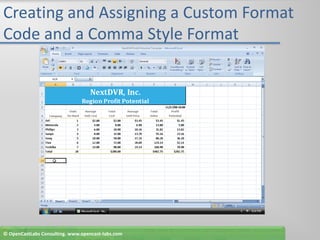
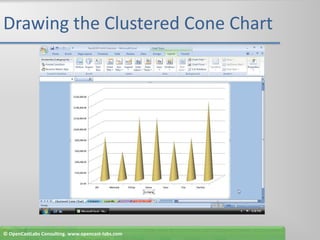
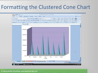
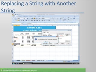
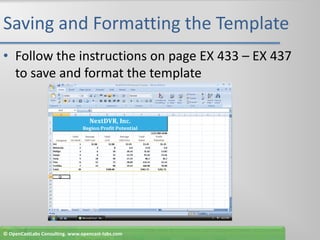
The document describes steps to format a worksheet template in Excel: 1. Margins were changed, headers and footers were added, and the printout was centered horizontally on the page. 2. A custom format code was created and applied to cells, and a new cell style was defined and applied. 3. Formulas using 3D references were entered and copied to other cells, and a clustered cone chart was drawn and formatted on a separate sheet.

1. Excel Chapter 6Creating Templates and Working with Multiple Worksheets and Workbooks

2. ObjectivesCreate and use a templateUse the ROUND functionUtilize custom format codesDefine, apply, and remove a styleAdd a worksheet to a workbookCreate formulas that use 3-D cell referencesDraw a Clustered Cone chart© OpenCastLabs Consulting. www.opencast-labs.com

3. ObjectivesUse WordArt to create a title and create and modify shapesAdd a header or footer, change margins, and insert and move a page breakSave a workbook as a PDF or XPS fileUse the Find and Replace commandsCreate a workspaceConsolidate data by linking workbooks© OpenCastLabs Consulting. www.opencast-labs.com

4. Entering Formulas Using Point Mode and Determining Totals in the TemplateFollow the instructions on pages EX 423 – EX 427 to start Excel and prepare the TemplateSelect cell D5, type = to start the formula, click cell B5, type * (asterisk), click cell C5, and then click the Enter box in the formula barSelect cell E5, type =round(c5/(1-.42),2), and then click the Enter box in the formula bar to display the formula =ROUND(C5/(1-0.42), 2) in the formula bar and the value 3.45 (3.448276 rounded to two decimal places) as the average unit price in cell E5Follow the instructions on pages EX 430 – EX 432 to finish entering formulas and values into the worksheet© OpenCastLabs Consulting. www.opencast-labs.com

5. Entering Formulas Using Point Mode and Determining Totals in the Template© OpenCastLabs Consulting. www.opencast-labs.com

6. Saving and Formatting the TemplateFollow the instructions on page EX 433 – EX 437 to save and format the template© OpenCastLabs Consulting. www.opencast-labs.com

7. Creating and Assigning a Custom Format Code and a Comma Style FormatSelect the range C6:G11, right-click the selected range, and then click Format Cells on the shortcut menuWhen Excel displays the Format Cells dialog box, if necessary, click the Number tab, and then click Custom in the Category listIf necessary, scroll down and then click #,##0.00_); [Red](#,##0.00) in the Type listIn the Type text box, change the word Red to Blue© OpenCastLabs Consulting. www.opencast-labs.com

8. Creating and Assigning a Custom Format Code and a Comma Style FormatClick the OK button to display the numbers in the range C6:G11 using the custom format code created in Step 1Select the range B5:B12, click the Comma Style button on the Ribbon, and then click the Decrease Decimal button on the Ribbon twice to display the numbers in the range B5:B12 using the Comma style format with no decimal placesSelect cell A14© OpenCastLabs Consulting. www.opencast-labs.com

9. Creating and Assigning a Custom Format Code and a Comma Style Format© OpenCastLabs Consulting. www.opencast-labs.com

10. Creating a New StyleClick the Cell Styles button on the Home tab on the Ribbon to display the Cell Styles galleryClick the New Cell Style button in the Cell Styles galleryWhen Excel displays the Style dialog box, type Four-Digit Year as the new style nameClick the Format button to display the Format Cells dialog box© OpenCastLabs Consulting. www.opencast-labs.com

11. Creating a New StyleWhen Excel displays the Format Cells dialog box, if necessary, click the Number tab, click Date in the Category list, and then click 14-Mar-2001 in the Type listClick the Alignment tab, click the Horizontal box arrow, click Center in the Horizontal list, and then click the OK buttonWhen the Style dialog box becomes active, click Font, Border, Fill, and Protection to clear the check boxesClick the OK button to add the new Four-Digit Year style to the list of styles available with the NextDVR Profit Potential Template file in the Cell Styles gallery© OpenCastLabs Consulting. www.opencast-labs.com

12. Creating a New Style© OpenCastLabs Consulting. www.opencast-labs.com

13. Applying a New StyleSelect cell G3 and then click the Cell Styles button on the Ribbon to display the Cell Styles galleryClick the Four-Digit Year style to assign the Four-Digit Year style to cell G3 (Figure 6–29)Select cell A14© OpenCastLabs Consulting. www.opencast-labs.com

14. Applying a New Style© OpenCastLabs Consulting. www.opencast-labs.com

15. Opening a Template and Saving It as a WorkbookFollow the instructions on page EX 444 to spell check, print, and save the documentWith Excel active, click the Office Button and then click Open on the Office Button menuWhen Excel displays the Open dialog box, select UDISK 2.0 (E:) in the Address barClick the file name NextDVR Profit Potential Template to select itClick the Open button in the Open dialog box© OpenCastLabs Consulting. www.opencast-labs.com

16. Opening a Template and Saving It as a WorkbookWhen Excel displays the NextDVR Profit Potential Template, click the Office Button and then click Save As on the Office Button menuWhen the Save As dialog box appears, type NextDVR Profit Potential in the File name boxClick the Save as type box arrow and then click Excel WorkbookClick the Save button in the Save As dialog box to save the workbook© OpenCastLabs Consulting. www.opencast-labs.com

17. Opening a Template and Saving It as a Workbook© OpenCastLabs Consulting. www.opencast-labs.com

18. Adding a Worksheet to a WorkbookClick the Sheet2 tab at the bottom of the window and then click the Insert Cells button arrow on the Home tab on the Ribbon to display the Insert menuClick Insert Sheet to add a fourth worksheet named Sheet 4 between Sheet 1 and Sheet 2© OpenCastLabs Consulting. www.opencast-labs.com

19. Adding a Worksheet to a Workbook© OpenCastLabs Consulting. www.opencast-labs.com

20. Entering and Copying 3-D References Using the Paste Button MenuFollow the instructions on pages EX 449 – EX 455 to modify the worksheetsSelect cell B5 and then click the Sum button on the Ribbon to display the SUM function and ScreenTipClick the Louisville tab and then click cell B5. While holding down the SHIFT key, click the Portland tab to surround cell Louisville!B5 with a marqueeClick the Enter box in the formula bar to enter the SUM function with the 3-D references in cell Company!B5With cell B5 active, click the Copy button on the Ribbon to copy the SUM function and the formats assigned to cell B5 to the Office ClipboardSelect the range B6:B11 and then click the Paste button arrow on the Ribbon to display the Paste button menu© OpenCastLabs Consulting. www.opencast-labs.com

21. Entering and Copying 3-D References Using the Paste Button MenuClick Formulas on the Paste button menu to copy the SUM function in cell B5 to the range B6:B11 and automatically adjust the cell references in the SUM function to reference the corresponding cells on the three sheets in the workbookPress the ESC key to clear the marquee surrounding cell B5 and then select cell A14 to deselect the range B6:B11Click the Save button on the Quick Access Toolbar to save the NextDVR Profit Potential workbook© OpenCastLabs Consulting. www.opencast-labs.com

22. Entering and Copying 3-D References Using the Paste Button Menu© OpenCastLabs Consulting. www.opencast-labs.com

23. Drawing the Clustered Cone ChartWith the Company sheet active, select the range A5:A11Hold down the CTRL key and then select the range G5:G11Click the Insert tab on the RibbonClick the Column button on the Ribbon and then click Clustered Cone (column 1, row 4) in the Column gallery to insert a Clustered Cone chartClick the Move Chart button on the Ribbon© OpenCastLabs Consulting. www.opencast-labs.com

24. Drawing the Clustered Cone ChartWhen Excel displays the Move Chart dialog box, click New sheet and then type Clustered Cone Chart as the sheet nameClick the OK button in the Move Chart dialog box to move the chart to a new sheetClick the Layout tab on the Ribbon and then click the 3-D Rotation button on the Ribbon to display the Format Chart Area dialog boxType 70 in the X text box in the Rotation area to rotate the chart 70% along the X-axisType 30 in the Y text box in the Rotation area to rotate the chart 30% along the Y-axis© OpenCastLabs Consulting. www.opencast-labs.com

25. Drawing the Clustered Cone ChartClick the Close button in the Format Chart Area dialog boxClick the Legend button on the Ribbon and then click None to remove the legend from the right side of the chartClick the Axis Titles button on the Ribbon to display the Axis Titles menuPoint to Primary Horizontal Axis Title on the Axis Titles menu and then click Title Below Axis in the Primary Horizontal Axis Title gallery to add a title to the horizontal axisSelect the horizontal axis title and type Company as the new title© OpenCastLabs Consulting. www.opencast-labs.com

26. Drawing the Clustered Cone Chart© OpenCastLabs Consulting. www.opencast-labs.com

27. Formatting the Clustered Cone ChartRight-click the Clustered Cone Chart sheet tab, point to Tab Color on the shortcut menu, and then click Aqua, Accent 3 (column 7, row 1) on the Color paletteIf necessary, drag the tab split box (Figure 6–55) to the right to ensure all five tabs show. Drag the Clustered Cone Chart sheet tab to the right of the Portland sheet tabClick the chart wall behind the cones, click the Home tab on the Ribbon, click the Fill Color button arrow on the Ribbon, and then click Lavender, Accent 5, Lighter 40% (column 9, row 4) on the Fill Color palette© OpenCastLabs Consulting. www.opencast-labs.com

28. Formatting the Clustered Cone ChartClick the floor of the chart below the cones, click the Fill Color button arrow on the Ribbon, and then click White, Background 1, Darker 15% (column 1, row 3) on the Fill Color paletteClick one of the cylinders to select all the cones, click the Fill Color button arrow on the Ribbon, and then click Aqua, Accent 3 (column 7, row 1) on the Fill Color paletteClick the x-axis and then click the Bold button on the Ribbon. Click the y-axis and then click the Bold button on the Ribbon. Click outside the chart area to display the chart as shown on the following slide© OpenCastLabs Consulting. www.opencast-labs.com

29. Formatting the Clustered Cone Chart© OpenCastLabs Consulting. www.opencast-labs.com

30. Adding a Chart Title Using the WordArt ToolWith the Clustered Cone Chart sheet active, click anywhere on the chart, and then click the Insert tab on the RibbonClick the WordArt button on the Ribbon to display the WordArt galleryWhen Excel displays the WordArt gallery, point to the Gradient Fill – Accent 4, Reflection (column 5, row 4) selection in the WordArt galleryClick the Gradient Fill – Accent 4, Reflection selection in the WordArt gallery to insert a new WordArt objectWhen Excel displays the WordArt object on the chart, type Profit Potential as the title of the Clustered Cone chart© OpenCastLabs Consulting. www.opencast-labs.com

31. Adding a Chart Title Using the WordArt ToolSelect the text in the WordArt object to display the Mini toolbarClick the Font Size box arrow on the Mini toolbar and then click 44 in the Font Size list to change the font size of the WordArt object to 44Drag the top edge of the WordArt object so that the object is positioned above the cones in the chart as shown in Figure 6–60Click outside the chart area to deselect the WordArt object© OpenCastLabs Consulting. www.opencast-labs.com

32. Adding a Chart Title Using the WordArt Tool© OpenCastLabs Consulting. www.opencast-labs.com

33. Adding a Text Box, Arrow, and Brace to the ChartClick the Insert tab on the RibbonClick the Shapes button on the Ribbon to display the Shapes galleryClick the Text Box button (column 1, row 1) in the Shapes gallery to select itPoint to the upper-left corner of the planned text box location, and then drag the crosshair to the lower-right cornerWith the insertion point active in the text box, type Greatest Profit Potential as the text to display in the text box as shown in Figure 6–63© OpenCastLabs Consulting. www.opencast-labs.com

34. Adding a Text Box, Arrow, and Brace to the ChartClick the Insert tab on the Ribbon, click the Shapes button on the Ribbon, and then click the Left Brace button in the Shapes gallery (column 4, row 2)Point to the bottom-left corner of the Toshiba cone and then drag up to the top of the Toshiba cone and then slightly to the left to draw the braceClick the Subtle Line - Dark 1 shape style in the Shape Styles group to select it and change the color of the braceClick the Insert tab on the Ribbon, click the Shapes button on the Ribbon, and then click the Arrow button in the Shapes gallery (column 3, row 1)© OpenCastLabs Consulting. www.opencast-labs.com

35. Adding a Text Box, Arrow, and Brace to the ChartPoint immediately to the right of the letter t in Profi t in the text box, and then drag the arrow to the center of the brace to draw the arrowClick the Subtle Line - Dark 1 shape style in the Shape Styles group to select it and change the color of the braceClick outside the chart area to deselect the chartClick the Company tab and then select cell A14 to deselect the chart rangeClick the Save button on the Quick Access Toolbar to save the workbook© OpenCastLabs Consulting. www.opencast-labs.com

36. Adding a Text Box, Arrow, and Brace to the Chart© OpenCastLabs Consulting. www.opencast-labs.com

37. Adding a Header and Footer, Changing Margins, and Centering the Printout HorizontallyWith the Company sheet active, scroll to the top of the documentWhile holding down the SHIFT key, click the Portland sheet tab to select the four worksheet tabsClick the Page Layout tab on the RibbonClick the Page Setup Dialog Box Launcher to display the Page Setup dialog boxWhen Excel displays the Page Setup dialog box, if necessary, click the Margins tab© OpenCastLabs Consulting. www.opencast-labs.com

38. Adding a Header and Footer, Changing Margins, and Centering the Printout HorizontallyDouble-click the Top box and then type 1.5 to change the top margin to 1.5 inchEnter .5 in both the Left box and Right box to change the left and right margins to .5 inchClick the Horizontally check box in the ‘Center on page’ area to select it. This will center the worksheet on the page horizontallyClick the OK button in the Page Setup dialog box to close itClick the Page Layout button on the status bar to display the worksheet in Page Layout view© OpenCastLabs Consulting. www.opencast-labs.com

39. Adding a Header and Footer, Changing Margins, and Centering the Printout HorizontallyIf necessary, scroll the worksheet up until the Header area is displayed. Click the left Header box, type J. Quasney(or your name if you are stepping through the chapter on a computer), press the ENTER key, and then type Profit Potential to complete the entryClick the center section box and then click the Sheet Name button on the Ribbon to instruct Excel to insert the sheet name that appears on the sheet tab as part of the headerClick the right Header box, click the Current Date button on the Ribbon, press the COMMA key, press the SPACEBAR, and then click the Current Time button on the Ribbon to insert the date and time in the HeaderScroll the workbook down to view the Footer areaClick the middle section box, type Page, press the SPACEBAR, click the Page Number button on the Ribbon, press the SPACEBAR, type of, press the SPACEBAR, and then click the Number of Pages button on the Ribbon to add the footer© OpenCastLabs Consulting. www.opencast-labs.com

40. Adding a Header and Footer, Changing Margins, and Centering the Printout HorizontallyClick anywhere on the worksheet to deselect the page footerClick the Normal view button on the status bar and then select cell A14. Click the Page Layout tab on the Ribbon and then click the Page Setup Dialog Box Launcheron the Ribbon to display the Page Setup dialog boxClick the Print Preview button in the Page Setup dialog box to preview the Company sheetClick the Next Page button and Previous Page button on the Print Preview tab on the Ribbon to preview the other pagesAfter previewing the printout, click the Close Print Preview button on the Ribbon© OpenCastLabs Consulting. www.opencast-labs.com

41. Adding a Header and Footer, Changing Margins, and Centering the Printout Horizontally© OpenCastLabs Consulting. www.opencast-labs.com

42. Inserting and Removing a Page BreakFollow the instructions on pages EX 475 to EX 477 to add a header to the chart sheet and print the workbookWith the Company sheet active, select cell B12 and then click the Page Layout tab on the RibbonClick the Breaks button on the Ribbon and then click Insert Page Break on the Breaks menu to insert a page breakWith cell B12 active, click the Breaks button on the Ribbon to display the Breaks menuClick Remove Page Break to remove the page breaks© OpenCastLabs Consulting. www.opencast-labs.com

43. Inserting and Removing a Page Break© OpenCastLabs Consulting. www.opencast-labs.com

44. Hiding Page BreaksClick the Office Button and then click the Excel Options button on the Office Button menuWhen Excel displays the Excel Options dialog box, click the Advanced button to display Advanced Excel optionsScroll the window until the ‘Display options for this worksheet’ area appearsClick the ‘Show page breaks’ check box to clear the check boxClick the OK button to hide the page breaks as shown on the following slide© OpenCastLabs Consulting. www.opencast-labs.com

45. Hiding Page Breaks© OpenCastLabs Consulting. www.opencast-labs.com

46. Finding a StringClick the Home tab on the RibbonWith the Company sheet active, click the Find & Select button on the RibbonClick FindWhen Excel displays the Find and Replace dialog box, click the Options button so that it appears as shown in Figure 6–78 on page EX 482© OpenCastLabs Consulting. www.opencast-labs.com

47. Finding a StringType Toshiba in the Find what box, click the Within box arrow, select Workbook, and then click the Match case and ‘Match entire cell contents’ check boxes to select themClick the Find Next button to cause Excel to begin the search at cell A1 on the Company sheet and make cell A11 the active cell because it is the first cell to match the search stringContinue clicking the Find Next button to find the string, Toshiba, on the other sheets in the workbookClick the Close button in the Find and Replace dialog box to terminate the process and close the Find and Replace dialog box© OpenCastLabs Consulting. www.opencast-labs.com

48. Finding a String© OpenCastLabs Consulting. www.opencast-labs.com

49. Replacing a String with Another StringWith the Company sheet active, click the Find & Select button on the Ribbon and then click ReplaceWhen Excel displays the Find and Replace dialog box, type Philips in the Find what box and Royal Philips in the Replace with boxClick the Format button to the right of the Replace with box. When Excel displays the Replace Format dialog box, click the Font tab, click the Color box arrow, click Red (column 2, row 1 in the Standard colors area), click Italic in the Font style list, and then click the OK button.If necessary, click the Within box arrow and then click Workbook© OpenCastLabs Consulting. www.opencast-labs.com

50. Replacing a String with Another StringIf necessary, click the Match case and ‘Match entire cell contents’ check boxes to select themClick the Replace All button to replace the stringClick the OK button in the Microsoft Office Excel dialog boxClick the Close button in the Find and Replace dialog box© OpenCastLabs Consulting. www.opencast-labs.com

51. Replacing a String with Another String© OpenCastLabs Consulting. www.opencast-labs.com

52. Quitting ExcelClick the Close button on the right side of the Excel title barWhen Excel displays the Microsoft Office Excel dialog box, click the No button© OpenCastLabs Consulting. www.opencast-labs.com

53. Creating a Workspace FileFollow the instructions on pages EX 486 – EX 488 to search for and open the four NDVR workbooksWith the four NDVR workbooks opened and the Company Profit Potential workbook active, if necessary, click the View tab on the RibbonClick the Save Workspace button on the RibbonWhen Excel displays the Save Workspace dialog box, select UDISK 2.0 (E:) in the Address bar and then type NextDVR Workspace in the File name box© OpenCastLabs Consulting. www.opencast-labs.com

54. Creating a Workspace FileClick the Save button in the Save Workspace dialog box to save the file names of the workbooks open, of the workbooks displaying, and other display settingsIf the Microsoft Office Excel dialog box is displayed for any of the workbooks, click the No buttonClick the Office Button and then click the Exit Excel button on the Office Button menu to quit ExcelIf the Microsoft Office Excel dialog box is displayed for any of the workbooks, click the No button© OpenCastLabs Consulting. www.opencast-labs.com

55. Creating a Workspace File© OpenCastLabs Consulting. www.opencast-labs.com

56. Consolidating Data by Linking WorkbooksStart Excel as described on page EX 423. Click the Office Button and then click Open on the Office Button menu. When Excel displays the Open dialog box, select UDISK 2.0 (E:) in the Address bar. Double-click NextDVR Workspace to open the four workbooks saved in the workspace. Make NDVR Company Profit Potential the active worksheet. If necessary, double-click the NDVR Company Profit Potential window title bar to maximize itSelect cell B5. Click the Sum button on the Home tab on the Ribbon. Click the View tab on the Ribbon and then click the Switch Windows button arrow on the Ribbon. Click NDVR Louisville Profit Potential on the Switch Windows menu. Click cell B5. Delete the dollar signs ($) in the reference to cell B5 in the formula bar. Click immediately after B5 in the formula bar and then press the COMMA key© OpenCastLabs Consulting. www.opencast-labs.com

57. Consolidating Data by Linking WorkbooksClick the Switch Windows button arrow on the Ribbon and then click NDVR Kansas City Profit Potential. Select cell B5. Delete the dollar signs ($) in the reference to cell B5 in the formula bar. Click immediately after B5 in the formula bar and then press the COMMA keyClick the Switch Windows button arrow on the Ribbon and then click NDVR Portland Profit Potential. Select cell B5. Delete the dollar signs ($) in the reference to cell B5 in the formula bar. Click the Enter box.With cell B5 active in the NDVR Company Profit Potential workbook, drag the cell’s fill handle through cell B11. Select cell B5Click the Save button on the Quick Access Toolbar. If Excel displays a dialog box, select Overwrite changes. Click the OK button. Click the Office Button, click Print on the Office Button menu, and then click the OK button in the Print dialog box to print the workbook© OpenCastLabs Consulting. www.opencast-labs.com

58. Consolidating Data by Linking Workbooks© OpenCastLabs Consulting. www.opencast-labs.com

59. Closing All Workbooks at One Time and Quitting ExcelClick the Office Button and then click the Exit Excel button on the Office Button menuIf Excel displays the Microsoft Office Excel dialog box, click the No button© OpenCastLabs Consulting. www.opencast-labs.com

60. SummaryCreate and use a templateUse the ROUND functionUtilize custom format codesDefine, apply, and remove a styleAdd a worksheet to a workbookCreate formulas that use 3-D cell referencesDraw a Clustered Cone chart© OpenCastLabs Consulting. www.opencast-labs.com

61. SummaryUse WordArt to create a title and create and modify shapesAdd a header or footer, change margins, and insert and move a page breakSave a workbook as a PDF or XPS fileUse the Find and Replace commandsCreate a workspaceConsolidate data by linking workbooks© OpenCastLabs Consulting. www.opencast-labs.com

62. Excel Chapter 6 Complete