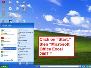
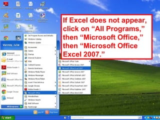
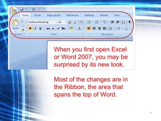
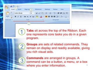
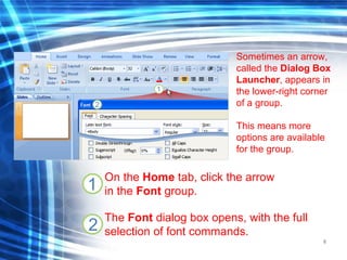
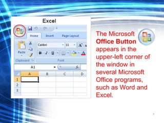
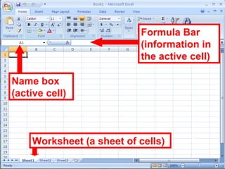
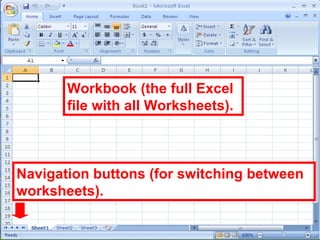
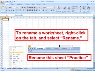
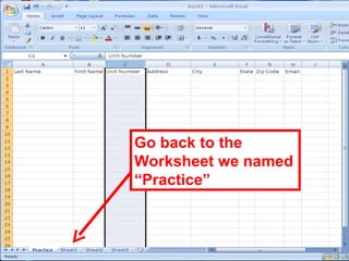
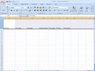
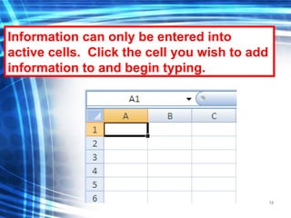
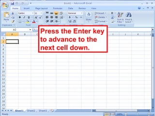
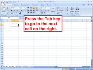
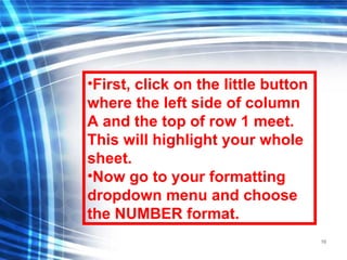
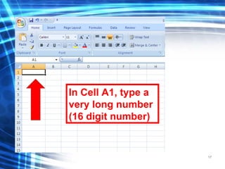
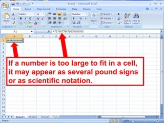
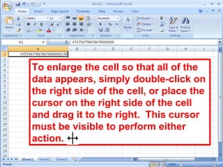
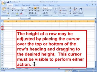
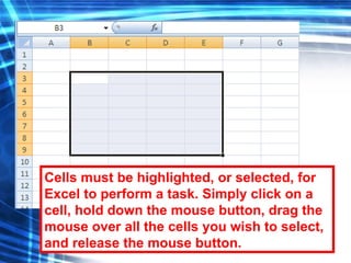
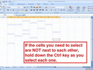
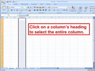
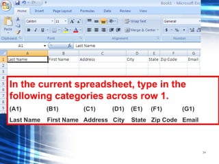
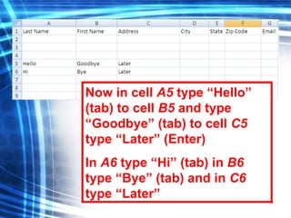
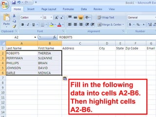
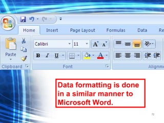
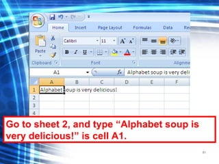
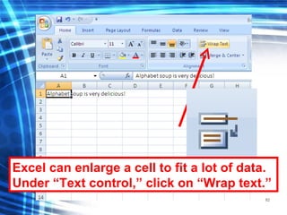
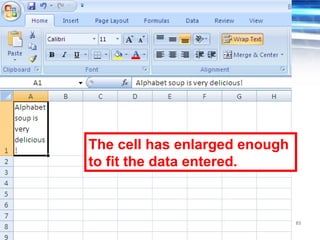
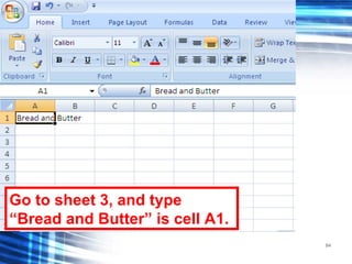
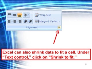
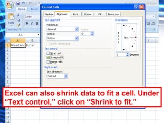
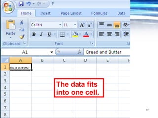
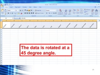
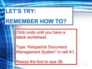
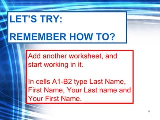
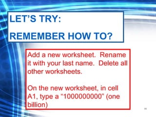
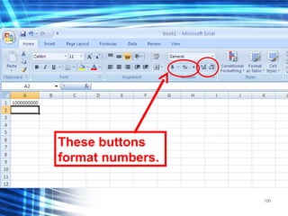
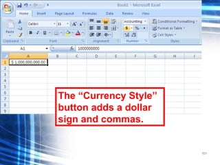
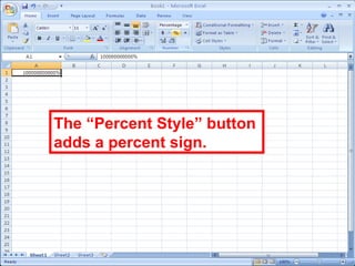
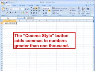
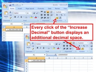
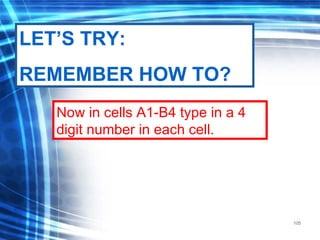
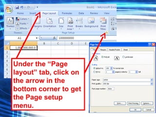
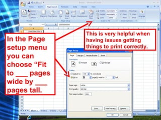
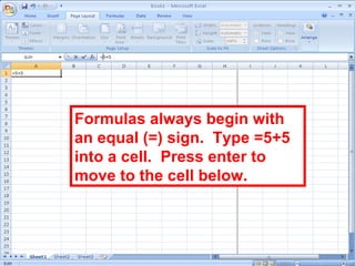
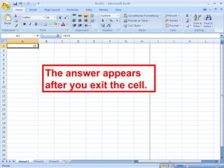
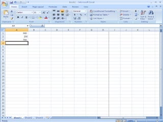
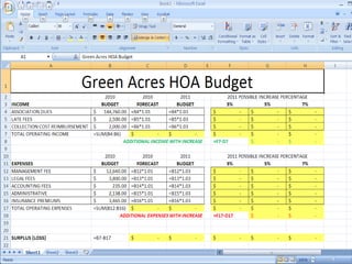
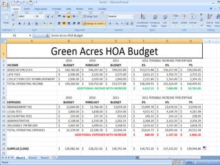
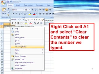
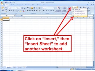
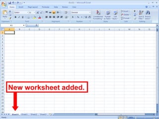
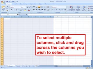
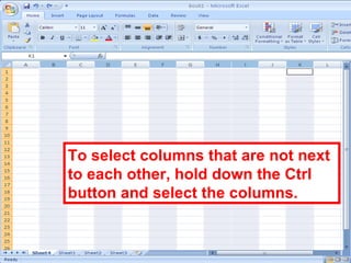
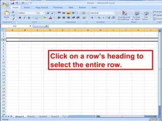
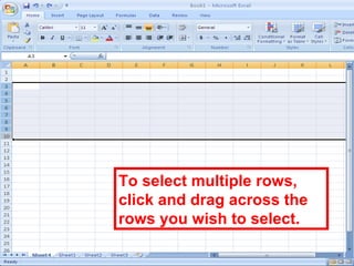
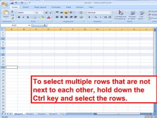
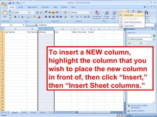
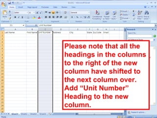
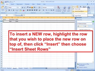
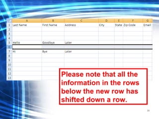
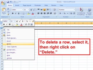
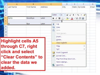
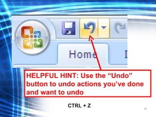
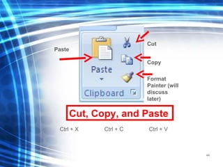
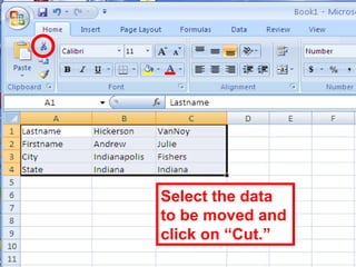
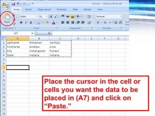
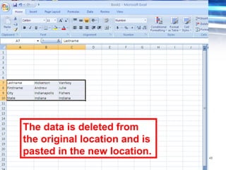
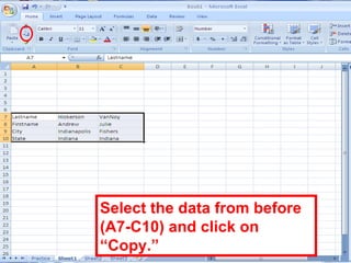
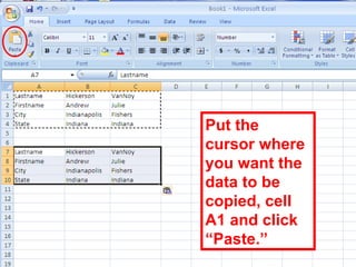
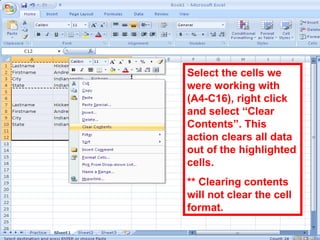
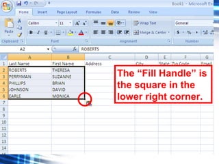
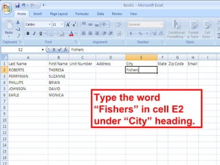
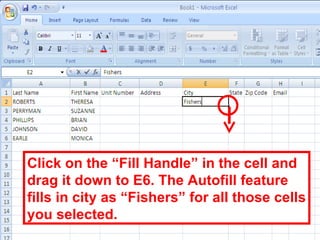
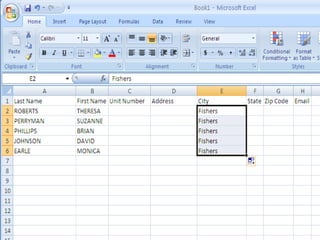
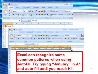
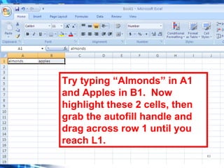
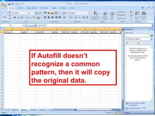
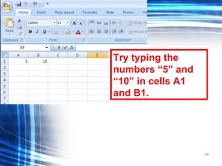
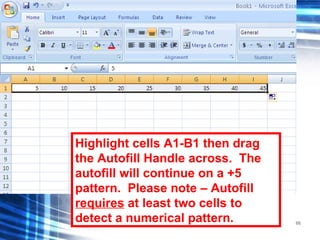
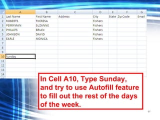
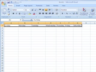
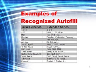
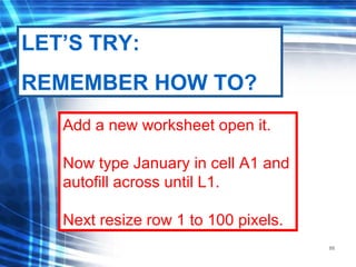
This document provides instructions for using basic Microsoft Excel functions including: 1) Opening Excel and navigating the ribbon interface and worksheet tabs 2) Entering and formatting data in cells, including adjusting cell size and formatting numbers 3) Common tasks like copying, cutting, pasting, inserting and deleting rows and columns 4) Using autofill to quickly populate cells with repeating values or a pattern 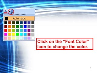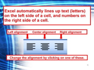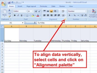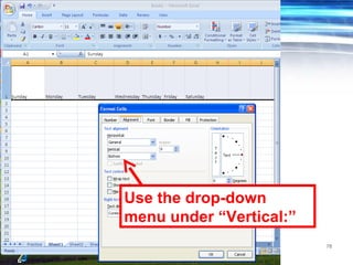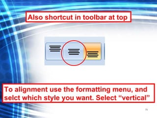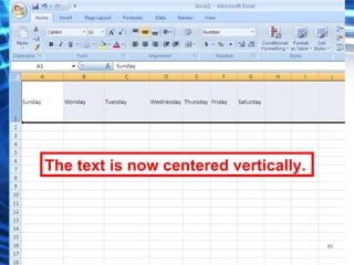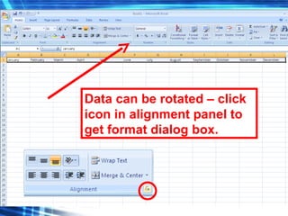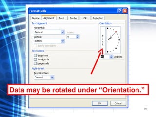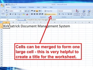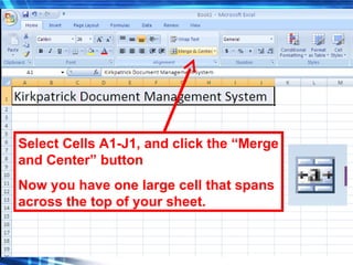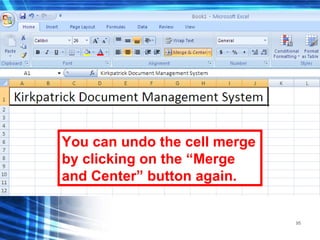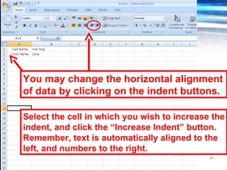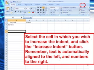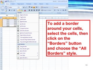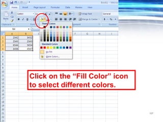5) Basic formatting options like font style, size, color, alignment, borders, and cell merges

1. 1
Microsoft Excel

2. 2
Click on “Start,”
then “Microsoft
Office Excel
2007.”

3. 3
If Excel does not appear,
click on “All Programs,”
then “Microsoft Office,”
then “Microsoft Office
Excel 2007.”

4. 4
When you first open Excel
or Word 2007, you may be
surprised by its new look.
Most of the changes are in
the Ribbon, the area that
spans the top of Word.

5. 5
1
2
3
Tabs sit across the top of the Ribbon. Each
one represents core tasks you do in a given
program.
Groups are sets of related commands. They
remain on display and readily available, giving
you rich visual aids.
Commands are arranged in groups. A
command can be a button, a menu, or a box
where you enter information.

6. 6
Sometimes an arrow,
called the Dialog Box
Launcher, appears in
the lower-right corner
of a group.
This means more
options are available
for the group.
1
2
On the Home tab, click the arrow
in the Font group.
The Font dialog box opens, with the full
selection of font commands.

7. 7
The Microsoft
Office Button
appears in the
upper-left corner of
the window in
several Microsoft
Office programs,
such as Word and
Excel.

8. 8
Let’s examine the
different areas of
the Excel
worksheet

9. 9
Each box
is called
a “cell.”
Column
headings
Row
headings

10. 10
Name box
(active cell)
Formula Bar
(information in
the active cell)
Worksheet (a sheet of cells)

11. 11
Workbook (the full Excel
file with all Worksheets).
Navigation buttons (for switching between
worksheets).

12. 12
Information can only be entered into
active cells. Click the cell you wish to add
information to and begin typing.

13. 13
Press the Enter key
to advance to the
next cell down.

14. 14
Press the Tab key
to go to the next
cell on the right.

15. 15
**Hitting enter and tab are
actually time savers. When
there is any action that you
can accomplish without taking
your hands off the keyboard,
you are actually saving a little
bit of time.

16. 16
•First, click on the little button
where the left side of column
A and the top of row 1 meet.
This will highlight your whole
sheet.
•Now go to your formatting
dropdown menu and choose
the NUMBER format.

17. 17
In Cell A1, type a
very long number
(16 digit number)

18. 18
If a number is too large to fit in a cell,
it may appear as several pound signs
or as scientific notation.

19. 19
To enlarge the cell so that all of the
data appears, simply double-click on
the right side of the cell, or place the
cursor on the right side of the cell
and drag it to the right. This cursor
must be visible to perform either
action.

20. 20
The height of a row may be
adjusted by placing the cursor
over the top or bottom of the
row’s heading and dragging to
the desired height. This cursor
must be visible to perform either
action.

21. 21

22. 22
Right Click cell A1
and select “Clear
Contents” to clear
the number we
typed.

23. 23
Click on “Insert,” then
“Insert Sheet” to add
another worksheet.

24. 24
New worksheet added.

25. 25
To rename a worksheet, right-click
on the tab, and select “Rename.”
Rename this sheet “Practice”

26. 26
Cells must be highlighted, or selected, for
Excel to perform a task. Simply click on a
cell, hold down the mouse button, drag the
mouse over all the cells you wish to select,
and release the mouse button.

27. 27
If the cells you need to select
are NOT next to each other,
hold down the Ctrl key as you
select each one.

28. 28
Click on a column’s heading
to select the entire column.

29. 29
To select multiple
columns, click and drag
across the columns you
wish to select.

30. 30
To select columns that are not next
to each other, hold down the Ctrl
button and select the columns.

31. 31
Click on a row’s heading to
select the entire row.

32. 32
To select multiple rows,
click and drag across the
rows you wish to select.

33. 33
To select multiple rows that are not
next to each other, hold down the
Ctrl key and select the rows.

34. 34
In the current spreadsheet, type in the
following categories across row 1.
(A1) (B1) (C1) (D1) (E1) (F1) (G1)
Last Name First Name Address City State Zip Code Email

35. 35
To insert a NEW column,
highlight the column that you
wish to place the new column
in front of, then click “Insert,”
then “Insert Sheet columns.”

36. 36
Please note that all the
headings in the columns
to the right of the new
column have shifted to
the next column over.
Add “Unit Number”
Heading to the new
column.

37. 37
Now in cell A5 type “Hello”
(tab) to cell B5 and type
“Goodbye” (tab) to cell C5
type “Later” (Enter)
In A6 type “Hi” (tab) in B6
type “Bye” (tab) and in C6
type “Later”

38. 38
To insert a NEW row, highlight the row
that you wish to place the new row on
top of, then click “Insert” then choose
“Insert Sheet Rows”

39. 39
Please note that all the
information in the rows
below the new row has
shifted down a row.

40. 40
To delete a row, select it,
then right click on
“Delete.”

41. 41
Highlight cells A5
through C7, right
click and select
“Clear Contents” to
clear the data we
added.

42. 42
HELPFUL HINT: Use the “Undo”
button to undo actions you’ve done
and want to undo
CTRL + Z

43. 43
Data can be moved around or
copied by using Cut, Copy, and
Paste.

44. 44
Cut, Copy, and Paste
Ctrl + X Ctrl + C Ctrl + V
Cut
Format
Painter (will
discuss
later)
Paste
Copy

45. 45
Go to Sheet 2, then fill in the following Information.
(A1) Lastname (B1) Hickerson (C1) VanNoy
(A2) Firstname (B2) Andrew (C2) Julie
(A3) City (B3) Indpls (C3) Fishers
(A4) State (B4) Indiana (C4) Indiana

46. 46
Select the data
to be moved and
click on “Cut.”

47. 47
Place the cursor in the cell or
cells you want the data to be
placed in (A7) and click on
“Paste.”

48. 48
The data is deleted from
the original location and is
pasted in the new location.

49. 49
Now try to cut and paste again
replacing the info in the original
spot.

50. 50
Using “Copy” and “Paste”
does not delete the data
from the original location,
but instead keeps the
original and the replica.

51. 51
Select the data from before
(A7-C10) and click on
“Copy.”

52. 52
Put the
cursor where
you want the
data to be
copied, cell
A1 and click
“Paste.”

53. 53
Select the cells we
were working with
(A4-C16), right click
and select “Clear
Contents”. This
action clears all data
out of the highlighted
cells.
** Clearing contents
will not clear the cell
format.

54. 54
Using Autofill

55. 55
Using AutoFill can save
work by copying data or
repeating patterns.

56. 56
Go back to the
Worksheet we named
“Practice”

57. 57
Fill in the following
data into cells A2-B6.
Then highlight cells
A2-B6.

58. 58
The “Fill Handle” is
the square in the
lower right corner.

59. 59
Type the word
“Fishers” in cell E2
under “City” heading.

60. 60
Click on the “Fill Handle” in the cell and
drag it down to E6. The Autofill feature
fills in city as “Fishers” for all those cells
you selected.

61. 61

62. 62
Excel can recognize some
common patterns when using
Autofill. Try typing “January” in A1
and auto fill until you reach K1.

63. 63
Try typing “Almonds” in A1
and Apples in B1. Now
highlight these 2 cells, then
grab the autofill handle and
drag across row 1 until you
reach L1.

64. 64
If Autofill doesn’t
recognize a common
pattern, then it will copy
the original data.

65. 65
Try typing the
numbers “5” and
“10” in cells A1
and B1.

66. 66
Highlight cells A1-B1 then drag
the Autofill Handle across. The
autofill will continue on a +5
pattern. Please note – Autofill
requires at least two cells to
detect a numerical pattern.

67. 67
In Cell A10, Type Sunday,
and try to use Autofill feature
to fill out the rest of the days
of the week.

68. 68

69. 69
Examples of
Recognized Autofill

70. 70
Now take a minute and try to autofill
on your own.
Any Questions?

71. 71
Formatting

72. 72
Data formatting is done
in a similar manner to
Microsoft Word.

73. 73
Click on the “Font Color”
icon to change the color.

74. 74
Excel automatically lines up text (letters)
on the left side of a cell, and numbers on
the right side of a cell.
Change the alignment by clicking on one of these.
Left alignment Center alignment Right alignment

75. 75
Resize Row 1 to 100 pixels. If
you have any questions,
please ask.
LET’S TRY:
REMEMBER HOW TO?

76. 76

77. 77
To align data vertically,
select cells and click on
“Alignment palette”

78. 78
Use the drop-down
menu under “Vertical:”

79. 79
To alignment use the formatting menu, and
selct which style you want. Select “vertical”
Also shortcut in toolbar at top

80. 80
The text is now centered vertically.

81. 81
Go to sheet 2, and type “Alphabet soup is
very delicious!” is cell A1.

82. 82
Excel can enlarge a cell to fit a lot of data.
Under “Text control,” click on “Wrap text.”

83. 83
The cell has enlarged enough
to fit the data entered.

84. 84
Go to sheet 3, and type
“Bread and Butter” is cell A1.

85. 85
Excel can also shrink data to fit a cell. Under
“Text control,” click on “Shrink to fit.”

86. 86
Excel can also shrink data to fit a cell. Under
“Text control,” click on “Shrink to fit.”

87. 87
The data fits
into one cell.

88. 88
Add a new worksheet open it.
Now type January in cell A1 and
autofill across until L1.
Next resize row 1 to 100 pixels.
LET’S TRY:
REMEMBER HOW TO?

89. 89
Data can be rotated – click
icon in alignment panel to
get format dialog box.

90. 90
Data may be rotated under “Orientation.”

91. 91
The data is rotated at a
45 degree angle.

92. 92
Click undo until you have a
blank worksheet.
Type “Kirkpatrick Document
Management System” in cell A1.
Resize the font to size 36.
LET’S TRY:
REMEMBER HOW TO?

93. 93
Cells can be merged to form one
large cell - this is very helpful to
create a title for the worksheet.

94. 94
Select Cells A1-J1, and click the “Merge
and Center” button
Now you have one large cell that spans
across the top of your sheet.

95. 95
You can undo the cell merge
by clicking on the “Merge
and Center” button again.

96. 96
Add another worksheet, and
start working in it.
In cells A1-B2 type Last Name,
First Name, Your Last name and
Your First Name.
LET’S TRY:
REMEMBER HOW TO?

97. 97
You may change the horizontal alignment
of data by clicking on the indent buttons.
Select the cell in which you wish to increase the
indent, and click the “Increase Indent” button.
Remember, text is automatically aligned to the
left, and numbers to the right.

98. 98
Select the cell in which you wish
to increase the indent, and click
the “Increase Indent” button.
Remember, text is automatically
aligned to the left, and numbers
to the right.

99. 99
Add a new worksheet. Rename
it with your last name. Delete all
other worksheets.
On the new worksheet, in cell
A1, type a “1000000000” (one
billion)
LET’S TRY:
REMEMBER HOW TO?

100. 100
These buttons
format numbers.

101. 101
The “Currency Style”
button adds a dollar
sign and commas.

102. 102
The “Percent Style” button
adds a percent sign.

103. 103
The “Comma Style” button
adds commas to numbers
greater than one thousand.

104. 104
Every click of the “Increase
Decimal” button displays an
additional decimal space.

105. 105
Now in cells A1-B4 type in a 4
digit number in each cell.
LET’S TRY:
REMEMBER HOW TO?

106. 106
To add a border
around your cells,
select the cells, then
click on the
“Borders” button
and choose the “All
Borders” style.

107. 107
Click on the “Fill Color” icon
to select different colors.

108. 108
Click on the “Font Color” button
to change the color of your data.

109. 109
Adjusting spreadsheets

110. 110
Click on Print Preview before
printing the worksheet. Dotted
lines will appear on the worksheet
after using Print Preview. The lines
indicate the page breaks.

111. 111
To get to the “Page
Setup” Menu, select
the Page Layout
Tab, then click the
small arrow in the
corner.

112. 112
You may
change the
Orientation,
adjust the
size of the
spreadsheet,
change the
margins, add
a
header/foote
r, and more.

113. 113
Various print options are
located on the “Print”
menu.

114. 114
Click on Print Preview before
printing the worksheet. Dotted
lines will appear on the worksheet
after using Print Preview. The lines
indicate the page breaks.

115. 115
Click on Print Preview before
printing the worksheet. Dotted
lines will appear on the worksheet
after using Print Preview. The lines
indicate the page breaks.

116. 116
Under the “Page layout” tab, you
can adjust the “Print area”. This is
the area that will be on the printed
copy of your spreadsheet.

117. 117
Under the “Page
layout” tab, click on
the arrow in the
bottom corner to get
the Page setup
menu.

118. 118
This is very helpful when
having issues getting
things to print correctly.
In the Page
setup menu
you can
choose “Fit
to ___ pages
wide by ___
pages tall.

119. 119
Basic Formulas

120. 120
Delete everything out of cells
A1-B4 so that you are working
from a blank worksheet.

121. 121
Formulas always begin with
an equal (=) sign. Type =5+5
into a cell. Press enter to
move to the cell below.

122. 122
The answer appears
after you exit the cell.

123. 123
If you go back to the
original cell, you will
see the formula in the
“Formula Bar.”

124. 124
Symbols
To add, use +
To subtract, use –
To multiply, use *
To divide, use /

125. 125
Excel calculates in
the following order:
Parentheses
Multiplication and
Division
Addition and
Subtraction

126. 126
Formulas can be
created based on
values in other cells.
The formula,
“=A1+A2” adds the
values in A1 and A2.

127. 127

128. 128
AutoSum

129. 129
In cells A1-A7 type a 3
digit number in each cell.

130. 130
AutoSum quickly adds the numbers in
cells. Simply highlight the numbers to be
added, then click on the AutoSum icon.
The answer will appear in the next cell.

131. 131
Click the small arrow
next to the AutoSum
icon to see other
functions available.

132. 132

133. 133
Error Messages
#DIV/0 (Dividing by 0)
#NAME? (Formula name or cell
reference is not recognized)
#REF! (Cell does not exist)
#VALUE! (A cell with text can NOT
work with formula)
####### (Appears when column is too
narrow to display results)

134. 134
Circular Reference Error

135. 135
The “Circular
Reference” error
appears when a
formula or function
refers to its own cell.

136. 136
For additional help with Excel,
including formulas and
functions, be sure to access
the “Help” menu.

137. 137
Practice Test

138. 138
Let’s create a fake budget for
a fake community.
Copy the following
information and try to get
formatting to match.

139. 139

140. 140
Now try to create the
formulas needed to
finish the spreadsheet.

141. 141
You will use”
=SUM( ) and XX*##

142. 142

143. 143
All highlighted cells need to
be solved with basic formulas.