This document provides an overview of Microsoft Excel. It discusses that Excel is a spreadsheet application used to organize data into tables and perform calculations. Key points covered include:
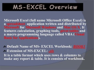
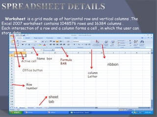
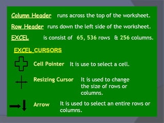
- Excel uses a grid of rows and columns to display data in worksheets.
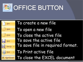
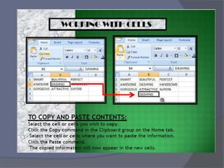
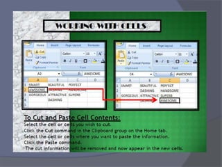
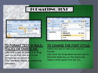
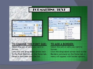
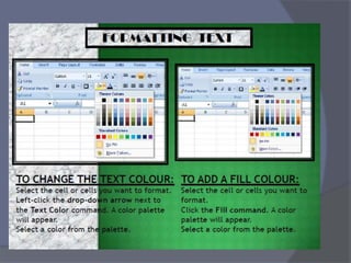
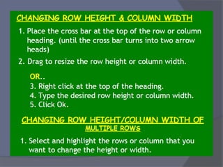
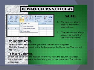
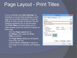
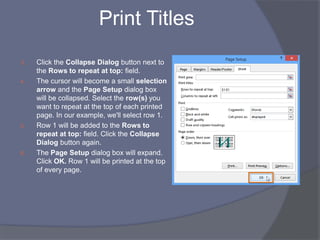
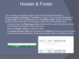
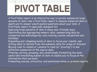
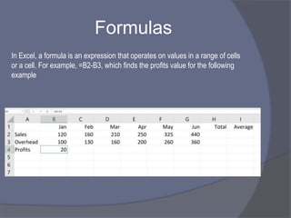
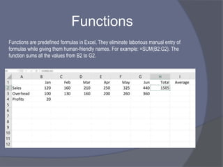
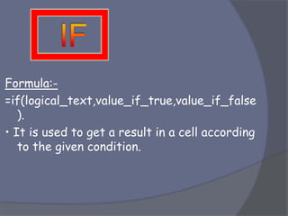
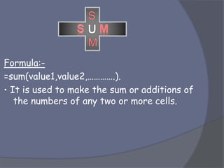
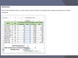
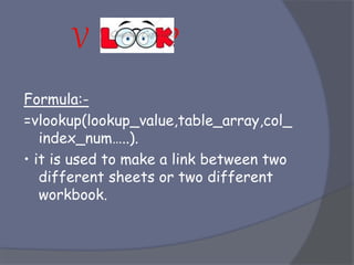
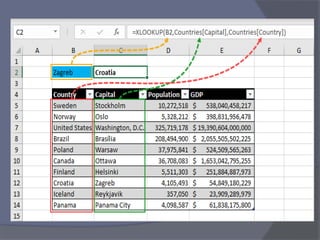
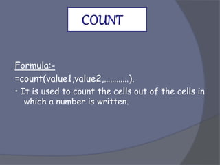
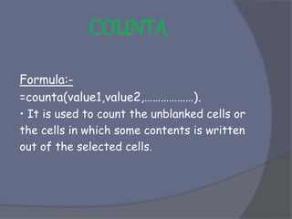
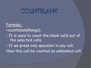
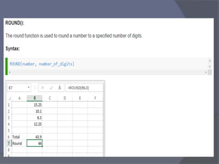
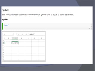
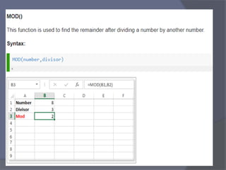
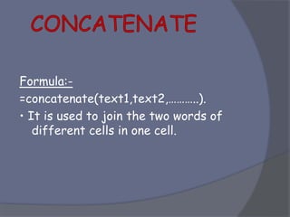
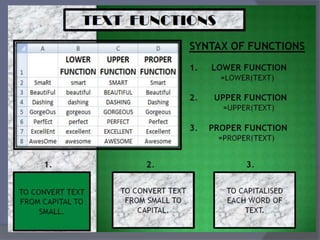
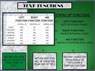
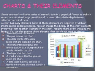
- Common tasks in Excel include entering data, formatting cells, adjusting worksheet layout, printing, using formulas and functions, and creating charts and pivot tables.
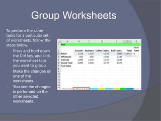
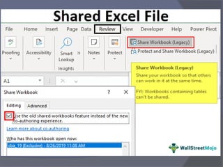
- Advanced features include conditional formatting, comments, grouping worksheets, and sharing workbooks with other users.


![20260201 [FOSDEM] gomodjail - library sandboxing for Go modules.pdf](https://cdn.slidesharecdn.com/ss_thumbnails/20260201fosdemgomodjail-librarysandboxingforgomodules-260201225659-76609ec4-thumbnail.jpg?width=640&height=640&fit=bounds)


