Downloaded 164 times
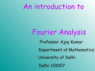
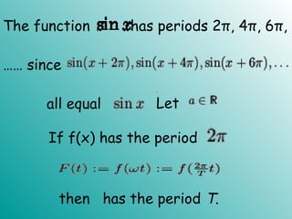

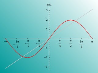
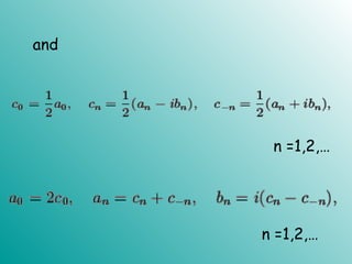
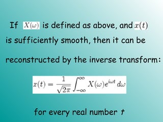
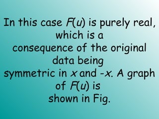
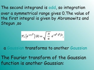
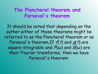
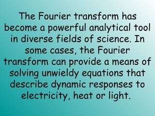
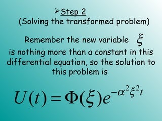
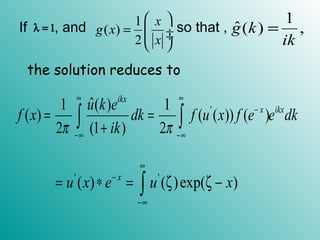
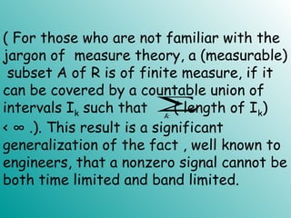
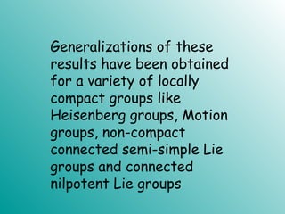
![would wonder how to define a similar
notion for functions which are L-periodic.
Assume that f(x) is defined and
integrable on the interval [-L,L]. Set
Remark.
We defined the Fourier series for
functions which are 2π -periodic, one](https://image.slidesharecdn.com/ft3new-101023025927-phpapp02/85/Ft3-new-18-320.jpg)
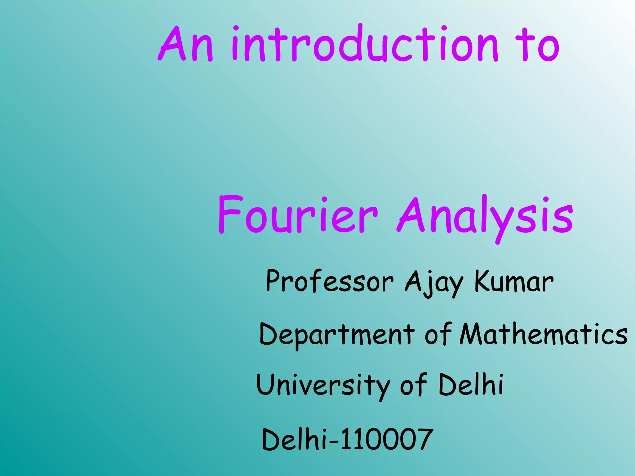
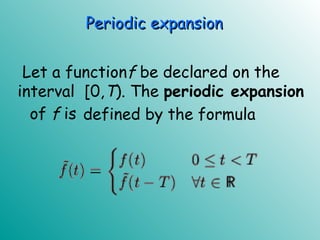
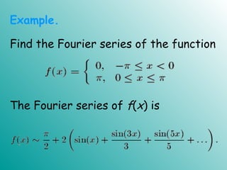
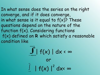
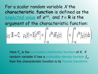
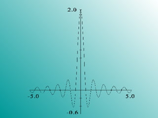
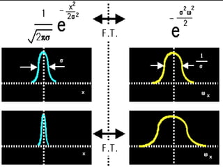
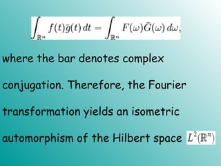
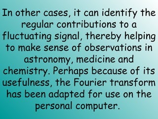
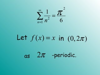
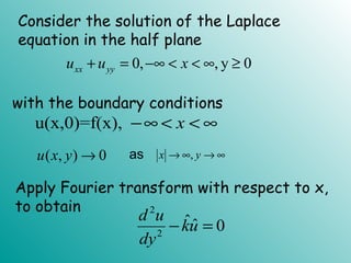
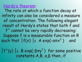
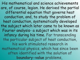
![The function F(x) is defined and
integrable on [-π , π ].Consider the Fourier
series of F(x)
Using the substitution,
we obtain the following definition:](https://image.slidesharecdn.com/ft3new-101023025927-phpapp02/85/Ft3-new-19-320.jpg)
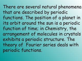
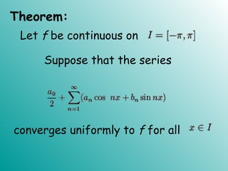
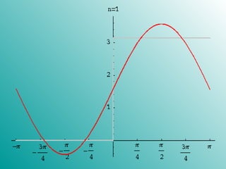
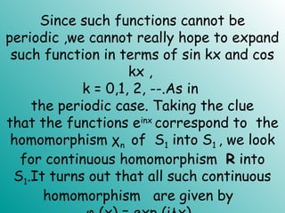
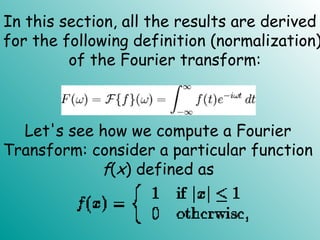
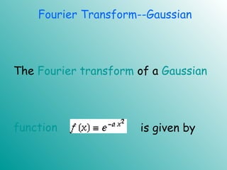
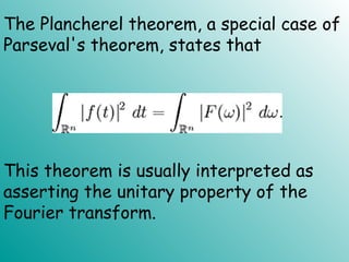
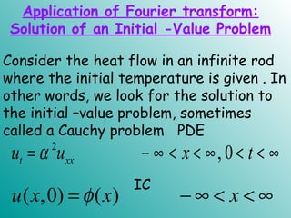
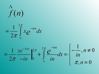
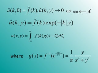
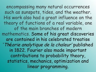
![Let f(x) be a function defined and integrable on
[-L,L]. The Fourier series of f(x) is
.
Definition.
for
where](https://image.slidesharecdn.com/ft3new-101023025927-phpapp02/85/Ft3-new-20-320.jpg)

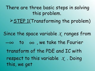
![2
[ ] [ ]
[ ( ,0)] [ ( )]
t xxF u F u
F u x F x
α
φ
=
=
and using the properties of the Fourier
transform, we have
2 2( )
( )
dU t
U t
dt
α ξ= −](https://image.slidesharecdn.com/ft3new-101023025927-phpapp02/85/Ft3-new-53-320.jpg)
![(0) ( )U ξ= Φ
is the Fourier transform ofΦ φ
( ) [ ( , )]U t F u x t=
where](https://image.slidesharecdn.com/ft3new-101023025927-phpapp02/85/Ft3-new-54-320.jpg)
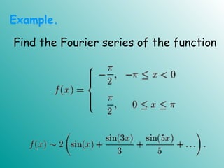
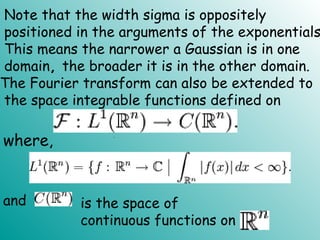
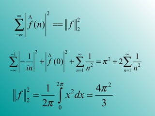
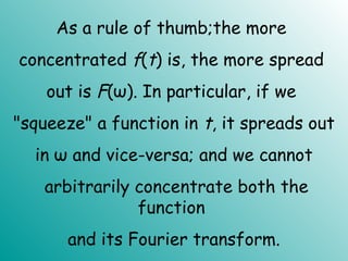
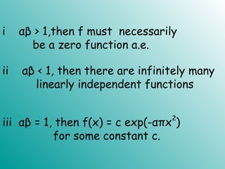
![
Step 3 (Finding the inverse transform)
To find the solution u(x,t) , we merely
compute
2 2
1 1
( , ) [ ( , )] [ ( ) ]t
u x t F U t F e α ξ
ξ ξ− − −
= = Φ
Now using one of the properties of
convolution, we get](https://image.slidesharecdn.com/ft3new-101023025927-phpapp02/85/Ft3-new-56-320.jpg)
![2 2
1 1
( , ) [ ( )] [ ]t
u x t F F e α ξ
ξ− − −
= Φ ∗
2 2
( / 4 )1
( )
2
x t
x e
t
α
φ
α π
−
= ∗
2 2
( ) / 41
( )
2
x t
e d
t
ξ α
φ ξ ξ
α π
∞
− −
−∞
= ∫
(using tables)
This is the solution to our problem.](https://image.slidesharecdn.com/ft3new-101023025927-phpapp02/85/Ft3-new-57-320.jpg)
![1
1 1 0
ˆˆ[ ( ) ( ) ( ) ] ( ) ( )n n
n na ik a ik a ik a y k f k−
−+ + − − − + + =
where
0
( )
n
r
r
r
P z a z
=
= ∑
ˆ( ) ˆ ˆˆ ˆ( ) ( ) ( ) ( )( )
( )
f k
y k f k q k f g k
P ik
= = = ∗
where
1
ˆ( )
( )
q k
P ik
=
( ) ( ) ( )y x f q x d
∞
−∞
= −∫ ζ ζ ζ
ˆˆ( ) ( ) ( )P ik y k f k=](https://image.slidesharecdn.com/ft3new-101023025927-phpapp02/85/Ft3-new-63-320.jpg)
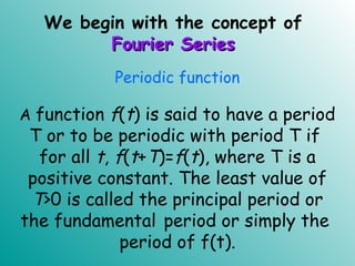
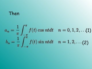
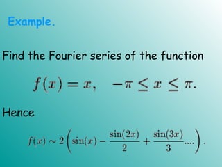
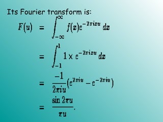
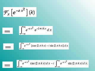
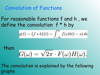
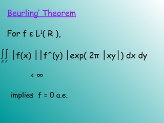
![( )
( ) sin
x
f x e
f x x
=
=
1
[ ] ( )
2
i x
F f f x e dxξ
π
∞
−
−∞
= ∫
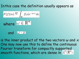
x → ∞
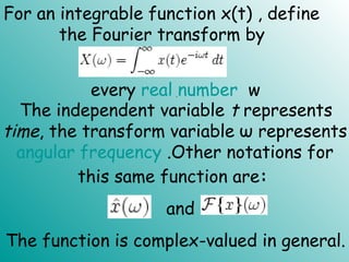
The major drawback of the Fourier
transform is that all functions can not be
transformed; for example, even simple
functions like
cannot be transformed, since the integral
does not exist. Only functions that
damp to zero sufficiently fast as
have transforms.](https://image.slidesharecdn.com/ft3new-101023025927-phpapp02/85/Ft3-new-73-320.jpg)


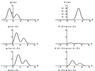
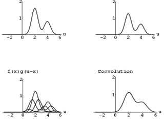
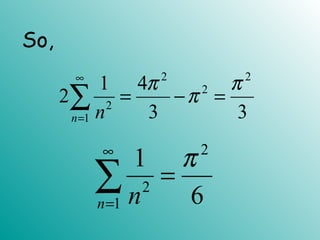
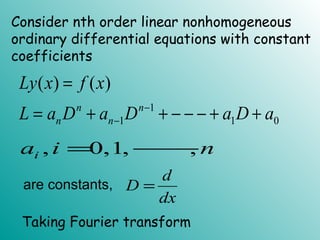
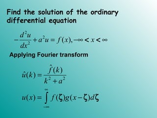
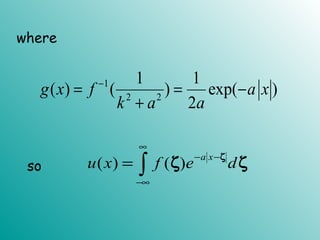
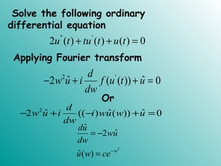
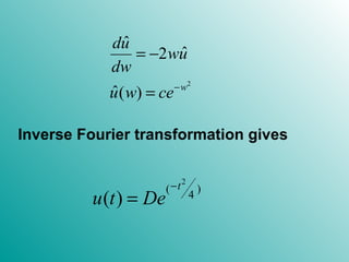
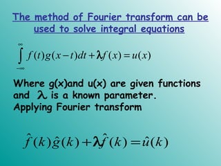
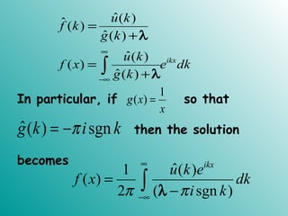
1. The document provides an introduction to Fourier analysis and Fourier series. It discusses how periodic functions can be represented as the sum of infinite trigonometric terms. 2. Examples are given of arbitrary functions being approximated by Fourier series of increasing lengths. As the length of the series increases, the ability to mimic the behavior of the original function also increases. 3. The Fourier transform is introduced as a method to represent functions in terms of sine and cosine terms. It allows problems involving differential equations to be transformed into an algebraic form and then transformed back to find the solution.