Downloaded 16 times


![The series approach has to be abandoned when the waveform is not pe-
riodic for example when Tp becomes infinite. As Tp increases the spacing
between 1/Tp = ω/2π decreases to dω/2π eventually becoming zero. The
discrete variable nω becomes continuos ω, and the amplitude and phase
spectra become continuos. This means that dn → d(ω) and Tp → ∞. With
these modifications we get the normalized formula [1],
dn = F(iω) =
1
2π
−∞
∞
f(t)e(−inωt)
dt. (10)
F(iω) is the complex Fourier integral,
F(iω) = Re(iω) + iIm(iω) = |F(iω)|eiφ(ω)
, (11)
where the amplitude is given by,
|F(iω)| = (Re(iω)2
+ Im(iω)2
)
1
2
(12)
and the phase by,
φ(w) = arctan[Im(iω)/Re(iω)]. (13)
|F(iω)| has the units of V Hz−1
.
The Fourier transform (FT) has very useful properties [2]. If f(x) has the
Fourier transform F(s), then f(ax) has the Fourier transform |a|−1
F(s/a).
Its application to waveforms and spectra is well known as compression of
the time scale corrensponds to expansion of the frequency scale. If f(x)
and g(x) have the Fourier transforms F(s) and G(s), then f(x) + g(x) has
F(s) + G(s) as the FT. The FT of f(x) is F(s), then f(x − a) has the FT
e−2πias
F(s). If f(x) has the FT F(s), then f(x) cos ωx has the FT 1
2
F(s −
ω/2π) + 1
2
F(s + ω/2π). If f(x) and g(x) have FTs F(s) and G(s), then
convolution f(x) ∗ g(x) has the FT F(s)G(s). The squarred modulus of a
function versus the squarred modulus of a spectrum yields;
∞
−∞
|f(x)|2
dx =
∞
−∞
|F(s)|2
ds. (14)
If f(x) has the FT F(s) then f′
(x) has the FT i2πF(s).
It can be seen from:
5](https://image.slidesharecdn.com/dippat-130510045604-phpapp01/85/Master-Thesis-on-Rotating-Cryostats-and-FFT-DRAFT-VERSION-7-320.jpg)
![∞
−∞
f′
(x)e−i2πxs
dx =
∞
−∞
lim
f(x + ∆x) − f(x)
∆x
e−i2πxs
dx = lim
∞
−∞
f(x + ∆x)
∆
e−i2πxs
dx − lim
∞
−∞
With these interesting properties let us turn to the discrete Fourier trans-
form (DFT) and the fast Fourier transform (FFT).
The digitalization of the analogue data requires the Fourier transforms
to be discrete. The analogue values are sampled at regular intervals and
then converted to binary representation. The operational viewpoint is that
it is irrelevant to talk about existence of values other than those given, and
those computed namely the input, and the output. Therefore we need the
mathematical theory to manipulate the actual quantified measurements.
Discreteness arises in connection with periodic functions. Discrete in-
tervals describing a periodic function may be viewed as a special case of
continuous frequency. This transform is thus regarded as equally spaced
deltafunctions multlipied by coeffients to determine their strengths.
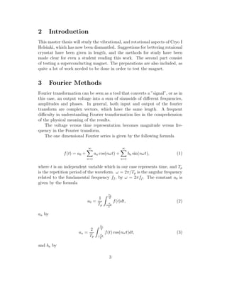
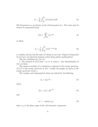
A typical fuction x(t) of the measurement is fed through an analogue to
digital converter. It samples x(t) at a series of regularly spaced times as
seen in Figure 1. Taking the sampling interval as ∆, then the discrete value
of x(t) = xr at time t is t = r∆, and can be written as a discrete time
sequence {xr}, r = . . . , −1, 0, 1, 2, 3, . . .. We are interested in the frequency
composition of sequence {xr} by analysis obtained from a finite length of
samples.
The historical method to estimate spectra from measured data was to
estimate an appropriate correlation function first and then to FT this func-
tion to obtain the required spectrum. This approach was until late 1960’s,
and practical calculations follewed the mathematical route of spectra defined
as FTs of correlation functions. The classical methods are studied in great
detail, and there is extensive literature ( [3], [4] and [5] on this subject.
The position was changed when fast Fourier transforms (FFT) came
along. This way of calculating the FT is much more efficient and faster.
Instead of determining a correlation function, and then calculating the FT,
FFT directly estimates the original FT of the time series.
If x(t) is a periodic function with period T, then it can be written:
x(t) = a0 + 2
α
k=1
ak cos(
2πkt
T
) + bk sin(
2πkt
T
) (16)
where k ≥ 0 is an integer, and
6](https://image.slidesharecdn.com/dippat-130510045604-phpapp01/85/Master-Thesis-on-Rotating-Cryostats-and-FFT-DRAFT-VERSION-8-320.jpg)
![Firstly we separate the odd and the even terms in {xr} getting
Xk =
1
N
N−1
r=0
xre−2iπkr/N
=
1
N
N/2−1
r=0
x2re−i2π(2r)k
N +
N/2−1
r=0
x2r+1e−i2π(2r+1)k
N =
1
N
N/2−1
r=0
yre−i2πrk
N/2 + e
from which
Xk =
1
2
Yk + e−i2πk/N
Zk , k = 0, 1, . . ., N/2 − 1. (34)
The original DFT can be obtained from Yk and Zk. If the original number
of samples is a power of 2, then the half-sequences {yr} and {zr} can be
partitioned into quarter-sequences, and so on, until the last sub-sequences
have only one term each. Yk and Zk are periodic and repeat themselves with
period N/2 so that Yk−N/2 = Yk and Zk−N/2 = Zk.
Calculating
Xk =
1
2
Yk + e−2iπk/N
Zk , k = 0, 1, . . ., N/2 − 1Xk =
1
2
Yk−N/2 + e−2iπk/N
Zk−N/2 , k = N/2, N/2 + 1
or
Xk =
1
2
Yk + e−2iπk/N
Zk Xk+N/2 =
1
2
Yk + e−2iπ(k+N/2)/N
Zk =
1
2
Yk − e−2iπk/N
Zk , k = 0, 1, . . ., N/
These are the formulas occuring in most FFT programs, and defining
W = e−2iπ/N
we obtain what is called coputational butterfly [6]. The FFT
changed the approach to digital spectral analysis when it was implemented
in 1965 ( [7] and [8]).
For general purposes Matlab’s FFT is used. It is based upon FFTW-
libraries [9]. FFTW uses several combinations of algorithms, including vari-
ation of the Cooley-Tukey algorithm, a prime factor algorithm [10], and a
split-radix algorithm [11]. The split-radix FFT requires N to be a power of
2 so the original sequence can be partitioned into two half-sequences of equal
length, and so on.
With these methods one is able to study the frequency depedence of the
input data. One should make the number of samples taken to be in the
form 2n
, where n is an integer. Even with number of samples the FFT
works quite some faster, for example a sequence that has N = 1048576 =
220
samples calculated directly with DFT compared to FFT has the ratio
11](https://image.slidesharecdn.com/dippat-130510045604-phpapp01/85/Master-Thesis-on-Rotating-Cryostats-and-FFT-DRAFT-VERSION-13-320.jpg)
![N2
/(N log2 N) = 52428, 8. Also one should make the sampling time interval
so small that the largest frequency that can be measured is well withing the
Nyquist frequency to avoid distortion due to aliasing. Otherwise if this is
not possible then filtering should be used in the experimental setup to cut
the frequency components above the Nyquist frequency to avoid aliasing.
4 Piezoelectric Accelerator
Piezoelectric effect was found in 1880 by Jaques and Pierre Curie in crys-
talline minerals, when subjected to a mechanical force the crystal became
electrically polarized. Compression and tension generated oppositely po-
larized voltages in proportion to the force. In converse if voltage-genarating
crystal was exposed to a electric field it contracted or expanded in accordance
with the polarity and field strength. These effects were called piezoelectric
effect and inverse piezoelectric effect. Quartz and other natural crystals
are widely used today in microphones, accelerometers, and ultrasonic trans-
ducers. Their applications include smart materials for vibration control,
aerospace, and astronautical applications of flexible surfaces, and vibration
reduction in sports equipment.
Consistent with the IEEE standards of piezoelectricity [12], the transduc-
ers are made of piezoelectric materials that are linear devices whose prop-
erties are governed by a set of tensor equations. To better understand the
workings of piezoelectricity we firstly turn to making of a piezoelectric ce-
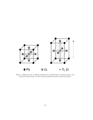
ramic crystal. A piezoelectric ceramic is a perovskite crystal composed of
a small tetravalent metal ion placed inside a larger lattice of divalent metal
ions and O2 (see Figure 3). Preparing such a ceramic, fine powders of the
component metal oxides are mixed in very specific proportions, and heated
to form a uniform powder, which is then mixed with an organic binder. The
powder turns into dense crystalline structure via specific process of heating,
and cooling.
Above the Curie temperature, each perovskite crystal exibit no dipole
moment (see Figure 4). Just below the Curie temperature each crystal has
tetragonal symmetry, and a dipole moment. Alaining these dipoles using
electrodes on the appropriate surfaces to create a strong DC electric field,
gives a net polarization. This is called poling process. After removing the
electric field most of the dipoles remain in a locked place, creating permanent
polarization and permanent elongation. The length increase of the element
is usually within the micrometer range. Tension or mechanical compression
changes the dipole moment associated with the particular element creating
a voltage. Tension perpendicular to direction of polarization or compression
12](https://image.slidesharecdn.com/dippat-130510045604-phpapp01/85/Master-Thesis-on-Rotating-Cryostats-and-FFT-DRAFT-VERSION-14-320.jpg)
![Figure 3: Crystalline structure of a piezoelectric crystal, before and after polarization.
along the direction of polarization generates voltage of the same polarity
as the poling voltalge. Tension along the polarization or compression per-
pendicular to the direction or polarization generates an opposite voltage to
that of the poling voltage. The voltage and the compressive stress generated
applying stress to the piezoelectric crystal are linearly proportional up to a
specific stress. In this way the crystal works as a sensor. The piezoelec-
tric crystal expands and contracts when poling voltages are applied, and in
this way the use is an actuator. This way electric energy is converted into
mechanical energy. When electric fields are low, and small mechanical stress
the piezoelectric materials have a linear profile. Under high stresses and elec-
tric fields this breaks into very nonlinear behavior. Straining mechanically a
poled piezoelectric crystal makes it electrically polarized, producing an elec-
tric charge on the surface of the material. This is the direct piezoelectric
effect and it is the basis of sensory use.
The electromechanical equations for a linear piezoelectric crystal are (
[12], [13]):
εi = SE
ij σj + dmiEm (37)
13](https://image.slidesharecdn.com/dippat-130510045604-phpapp01/85/Master-Thesis-on-Rotating-Cryostats-and-FFT-DRAFT-VERSION-15-320.jpg)
![The charge generated can be determined
q = D1 D2 D3
dA1
dA2
dA3
, (55)
where dA1, dA2 and dA3 are the differential electrode areas in the y − z,
x − z and x − y planes. The voltage generated VP is related to charge
VP =
q
CP
, (56)
where CP is the capacitator of the sensor. By measuring VP , the strain can
be calculated from the integral above. A calibrated piezoelectric accelerom-
eter is a sensor, and the voltage measured can then be used as measure or
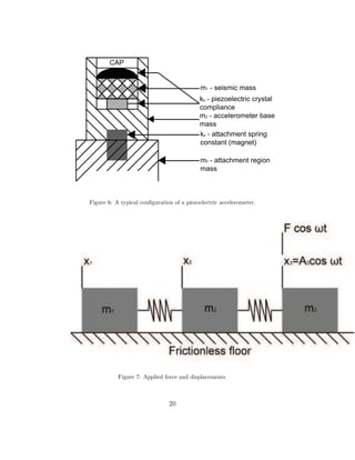
acceleration thus this is very useful for very precise frequency analysis. Fig-
ure 6 shows a typical configuration of a piezoelectric accelerometer mounted.
Small size, and rigidness generally means that stucture’s vibrational charac-
teristics will be minimal, but the structure does often affect the vibrational
characteristics of the attached accelerometer. Accelerometer’s sensitivity is
defined as the ratio of the output signal (voltage in our case) to the acceler-
ation of its base. The major resonant frequency of the accelerometer is the
lowest frequency for which the sensitivity has a maximum. The frequency
range of use is generally taken as that region in which sensitivity does not
change significantly from the value found near 100 Hz [14] when calibrated
on a conventional shaker table. The upper limit of an accelerometer is lower
than the determined by resonance of the accelerometer alone, when the mass
of accelerometer affects the motion of the structure.
To estimate the largest frequency to be measured can be calculated using
the following model. We assume the system consisting of masses (m1, m2 and
m3), and springs (assumed massless, and their spring constants ka and ks)
as in Figure 6. Let us suppose that a sinusoidally varying mechanical force
F cos ωt, is imposed on m3 from outside the system taking the position x3 is
A3 cos ωt. The resultant motion of m1, and m2 or the varying positions x1
and x2 (Figure 7) are considered as the frequency of the drive force is varied.
After transient effects die away, the equations describing the motion of m1
and m2 under the dynamic forces are:
m1 ¨x1 + ka(x1 − x2) = 0 (57)
m2 ¨x2 + ka(x2 − x1) + ks(x2 − x3) = 0. (58)
19](https://image.slidesharecdn.com/dippat-130510045604-phpapp01/85/Master-Thesis-on-Rotating-Cryostats-and-FFT-DRAFT-VERSION-21-320.jpg)
![The resonance sought is the lowest value of ω at which a maximum of
(x1 − x2) occurs by varying ω. When the system is in dynamic equilibrium
and resonance is approached from below, the motions will be at the drive
frequency and in phase.
x1 = A1 cos ωt (59)
x2 = A2 cos ωt (60)
¨x1 = −A1ω2
cos ωt (61)
From this we obtain
(ka − m1ω2
)A1 − kaA2 = 0 (62)
−kaA1 + (ks + ka − m2ω2
)A2 = ksA3 (63)
Resonance occurs when A1 − A2 has a maximum value. There’s no prob-
lem due to phase considerations because resonance is approached from below
and, with no damping, x1 and x2 can be considered to be in phase with the
motion of the driving element i.e. with x3. The solution for A1 and A2 each
has the determinant of its coefficients in the denominator. Thus maximum
values of A1 and A2 occur when this determinant vanishes. An equation in
the resonant frequency ω results:
(ka − m1ω2
)(ka + ks − m2ω2
) − k2
a = 0. (64)
This can be written as quadratic in ω2
,
ω4
− [ka(
1
m1
+
1
m2
) + ks
1
m2
]ω2
+
kaks
m1m2
= 0 (65)
Now we simplify the calculations by taking new constants a = m2/m1,
r = ks/ka, and ω2
0 = ka/m1. Substituting these into the above equation and
calculating the frequency:
ω = ω2
0
[1 + 1
a
(1 + r)] − [1 + 1
a
(1 + r)]2 − 4r
a
2
. (66)
21](https://image.slidesharecdn.com/dippat-130510045604-phpapp01/85/Master-Thesis-on-Rotating-Cryostats-and-FFT-DRAFT-VERSION-23-320.jpg)
![From this we can get the upper limit of the usable frequency. Usually this
value is given, and sometimes the relative frequency is given as ω/ω0. If this
value is not given, then one can estimate. Now in our case the measurements
on the cryostat imply that the mass of the accelerometer does not alter
the results, and the accelerometers base m2 is rigidly attached (in our case
a very strong magnet and straps) to a very large mass m3 (cryostat’s or
the supporting frame’s mass) so that m1 and ka are the only resonance-
determined parameters. These parameters are usually given, but if not it
can be relatively easy to approximate those. In this case of rigid attachment
masses m2 and m3 are combined, and taking m3 = ∞ we get
ω = ka/m1. (67)
The Nyquist frequency should be set little below this frequncy, and the all
frequencies above the Nyquist frequency should be filtered out (see next sec-
tion). Or if it is know what frequencies are to be looked for then the highest
frequency should be set according to that. Accelerometers are also subjected
to thermal-transient stimuli from stronger vibrations. Certain properties
of piezoelectric accelerometers can cause them to generate spurious output
signals in response to such thermal transients, leading to significant measure-
ment errors. Many piezoelectric crystalline materials are also pyroelectric [15]
that is, a change of temperature causes a change in the polarization charges
in the material. Pyroelectric output signals can result from a uniform or
non-uniform distribution of thermal charges within the material. In addi-
tion, mechanical strain within the piezoelectric element, resulting differential
thermal expansion of the components of an accelerometer subjected to ther-
mal transients, may generate spurious output signals. In conditions where
the accelerometer is exposed to blasts, non-uniform heating is propable. The
resultant output signal will thus include pyroelectrically generated charges
and charges produced by changes in the mechanical loading of the crystal
resulting from differential expansion of accelerometer components. This is
the reason why after rigid attaching of the piezoelectric accelerometer on the
cryostat or its frame one should wait for some time for normal conditions to
reappear. Usually the pyroelectric effect under normal stated conditions for
most piezoelectric crystals are not significant under frequencies of 3000 Hz
and amplitudes of 5 g [16]. So there should not be any problem with normal
measurements with the setup of the cryostat. However care should be taken
as to where the accelerometer is placed, e.g. it should not be placed in close
proximity of electronic devices that give strong electric fields or directly leak
heat into the surroundings.
22](https://image.slidesharecdn.com/dippat-130510045604-phpapp01/85/Master-Thesis-on-Rotating-Cryostats-and-FFT-DRAFT-VERSION-24-320.jpg)
![5 Low-pass filter and measurement setup
Taking into account the different frequency aspects namely the Nyquist fre-
quency, and the maximum frequency of the piezoelectric accelerometer under
which it operates, one needs to have a low-pass filter. Using this wisely will
eliminate almost all coputed aliasing, and bad signals from the crystal. Usu-
ally the window of interest lies somewhere in the region of 0 to 100 Hz, which
is easily attained by the machinery used. Ideally low-pass filters completely
eliminate all frequencies above the cut-off frequency while passing those be-
low unchanged. Real time filters approximate the ideal filter by windowing
the infinite impulse response to make a finete impulse response. Digital filter-
ing in our case is not the best solution, better is to use an electronic low-pass
filter. A second-order filter does a better job of attenuating higher frequen-
cies. There are many different types of filter circuits, with different responses
to changing frequency. A first-order filter will reduce the signal amplitude by
half every time the frequency doubles (goes up one octave). As the frequency
reach of the equipment used is so large, the low-pass filter can be relatively
simple one. One could use or build easily an active low-pass filter. In the
operational amplifier shown in the Figure 8, the cutoff frequency is defined
as
fc =
1
2πR2C
(68)
or equivalently in radians per second
ωc =
1
R2C
. (69)
The gain in the passband is −R2/R1, and the stopband drops off at −6dB
per octave, as it is a first-order filter.
If this doesn’t work as wished one can easily build a second order (or
higher) Butterworth filter (see Figure 9 [19]), which decreases −12dB per
octave. Also the frequency responce of the Butterworth filter is maximally
flat [18] in the passband compared to Chebyschev Type I / Type II or an
elliptic filter [17].
6 Vibrations
The types of vibrations in our case can be divided into two main categories:
the unbalanced rotation of the cryostat creates harmonic oscillations and
23](https://image.slidesharecdn.com/dippat-130510045604-phpapp01/85/Master-Thesis-on-Rotating-Cryostats-and-FFT-DRAFT-VERSION-25-320.jpg)
![Figure 8: An active low-pass filter.
Figure 9: Butterworth low-pass filter in a circuit used to obtain vibration spectra [19].
24](https://image.slidesharecdn.com/dippat-130510045604-phpapp01/85/Master-Thesis-on-Rotating-Cryostats-and-FFT-DRAFT-VERSION-26-320.jpg)
![other noisy vibrations, and other is resulting from external vibrations e.g.
electronic devices on the cryostat, the pumps and vibrations from ground
or foundation vibrations. Torsional vibration analysis is vital for ensuring
reliable machine operation, especially as very precise measurements are made
on the large cryostat. If rotating component failures occur on the cryostat
as a result of torsional oscillations, the consequences can be catastrophic.
In the worst case, the entire machine can be wrecked as a result of large
unbalancing forces, and worse injury to human beigns might be inflicted.
The foundation and electronics vibations are easier to allocate, but are big
enough to cause problems as vibrations could affect the nuclear stage and
the demagnetization solenoid creating a heat leak there as suggested by [19].
The level of vibration in a structure can be attenuated by reducing either the
excitation or the response of the structure to that excitation or both. These
could be relocating equipment, or isolating the structure from the exciting
force. The torsional vibrations can be reduced by balancing the load on the
rotating machinery. Real structures consist of an infinite number of elestically
connected masses and have infinite number of degrees of freedom. In reality
the motion is often such that only a few coordinates is needed to describe
the motion. The vibration of some structures can be analysed using a sigle
degree of freedom. Other motions may occur, but in our case for instance
for analysing the electric and foundation vibrations other vibrations can be
dimished, and electrical devices can be measured one at the time (to see more
comprehensive study [20]. A body of mass m is free to move along a fixed
horizontal surface attached to a spring k one end fixed. Displacement of the
mass is denoted by x, so giving this initial displacement x0, and letting go
we get:
¨x +
k
m
x = 0 (70)
giving
x = A cos ωt + B sin ωt, (71)
where A and B are constants, and ω is the circular frequency. Now with
x = x0 and t = 0 gives A = x0, and ˙x = 0 and t = 0 gives
x = x0 cos
k
m
t. (72)
25](https://image.slidesharecdn.com/dippat-130510045604-phpapp01/85/Master-Thesis-on-Rotating-Cryostats-and-FFT-DRAFT-VERSION-27-320.jpg)
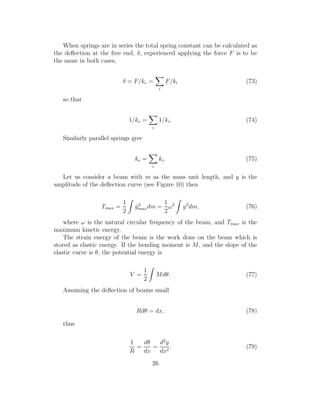
![Figure 10: Beam deflection.
From beam theory [21], M/I = E/R, where R is the radius of curvature
and EI is the flexural rigidity:
V =
1
2
M
R
dx =
1
2
EI
d2
y
dx2
2
dx. (80)
Now Tmax = Vmax;
ω2
=
EI d2y
dx2
2
dx
y2dm
. (81)
This expression gives the lowest natural frequency of transverse vibration
of a beam. It can be seen that to analyse the transverse vibration of a partic-
ular beam by this method requires y to be known as a function of x. In the
case of the cryostat’s frame this method can prove to be quite cumbersome.
Real structures dissipate vibration energy, so damping sometimes becomes
significant. Damping is difficult to model exactly because the mechanisms
of the structures. Using simplified models usually gain quite good results,
and can give insight to the problem. Viscous damping is a common form of
27](https://image.slidesharecdn.com/dippat-130510045604-phpapp01/85/Master-Thesis-on-Rotating-Cryostats-and-FFT-DRAFT-VERSION-29-320.jpg)
![When ζ = 1 the damping is critical and equation x = (A + Bt)e−ωt
is
valid. Finally damping greater than critical ζ > 1 gives two negative real
values of s so that x = X1es1t
+ X2es2t
. Substituting for damping constant
a constant friction force Fd that represents dry friction (Coulomb damping)
applicaple in many mechanisms:
m¨x + kx = Fd. (89)
Getting a solution
x = A sin ωt + B cos ωt +
Fd
k
. (90)
Hence
x = (x0 +
Fd
k
cos ωt +
Fd
k
, (91)
where the oscillation ceases with | x |≤ Fd/k, and the zone x = ±Fd/k is
called the dead zone. Many real structures have both viscous and Coulomb
damping. The two damping actions are sometimes dependent of amplitude,
and if the two cannot be separated a mixture of linear and exponential decay
functions have to be found by trial and error. In most real structures separat-
ing stiffness and damping effects is often not possible. This can be modeled
using complex stiffness k∗
= k(1 + iη), where k is the static stiffness, and
η is the hysteric damping loss factor. A range of values for η can be found
for common engineering materials in basic literature ( [22]). The electronic
devices on the cryostat behave as external excitation forces usually periodic.
From previous we construct a model as taking mass m connected to a fixed
spring and viscous damper, whilst a harmonic force of circular frequency ν
and amplitude F:
m¨x + c ˙x + kx = F sin(νt). (92)
Solution can be taken as x = X sin(νt − φ), where motion lags the force
by vector φ, so substituting and using cos − sin relations we get
mXν2
sin(νt − φ + π) + cXν sin(νt − φ + π/2) + kX sin(νt − φ) = F sin(νt).
(93)
29](https://image.slidesharecdn.com/dippat-130510045604-phpapp01/85/Master-Thesis-on-Rotating-Cryostats-and-FFT-DRAFT-VERSION-31-320.jpg)
![The force transmitted to the foundation is the sum of the spring force
and the damper force. Thus the transmitted force is given by
FT = (kX)2 + (cνX)2. (104)
The transmissibility is given by
TR =
FT
F
=
X k2 + (cν)2
F
(105)
since
X =
F/k
(1 − ν
ω
2
)2 + 2ζ ν
ω
)2
, (106)
TR =
1 + (2ζ ν
ω
)2
1 − (ν
ω
)2 + 2ζ ν
ω
2
. (107)
Therefore the force and motion transmissibilities are the same. It can be
seen that for good isolation ( [21]) ν/ω >
√
2, hence for a low value of ω
is required which implies a low stiffness, that is a flexible mounting. In the
cryostat it is particularly important to isolate vibration sources e.g. the elec-
trical devices because vibrations transmitted to structure radiate well, and
serious heat leak problems can occur. Theoretically low stiffness isolators
are desirable to gice a low natural frequency. There are four types of spring
material commonly used for resilient mountings and vibration isolation: air,
metal, rubber, and cork. Air springs can be used for very low-frequency
suspensions: resonance frequencies as low as 1 Hz can be achieved whereas
metal springs can only be used for resonance frequencies greater than about
1.3 Hz. Metal springs can transmit high frequencies, however, so rubber
or felt pads are often used to prohibit metal-to-metal contact between the
spring and the structure. Different forms of spring element can be used as
coil, torsion, cantilever and beam. Rubber can be used in shear or compres-
sion but rarely in tension. It is important to determine the dynamic stiffness
of a rubber isolator because this is generally much greater than the static
stiffness. Rubber also possesses some inherent damping although this may
be sensitive to amplitude, frequency and temperature. Natural frequencies
32](https://image.slidesharecdn.com/dippat-130510045604-phpapp01/85/Master-Thesis-on-Rotating-Cryostats-and-FFT-DRAFT-VERSION-34-320.jpg)
![from 5 Hz upwards can be achieved. Cork is one of the oldest materials
used for vibration isolation. It is usually used in compression and natural
frequencies of 25 Hz upwards are typical. For precise isolation systems, and
materials please refer to [23]. The above analysis is more for analysing the
vibrations due to electrical devices and the pumps, as they are consistent
usually having some periodicity giving only specific frequency peaks in fre-
quency spectrum. For external noise from the surroundings are more likely
to be random processes (as in [19]) possibly due to heavy traffic on a nearby
road or other large machinery used nearby. Collection of sample functions
x1(t), x2(t), . . . , xn(t), which make up the ensemble x(t). Normal or Gaussian
process is the most important of random processes because a wide range of
physically observed random waveforms represented by Gaussian process:
p(x) =
1
√
2πσ
e− 1
2
x−x
σ
2
, (108)
is the density function of x(t), where σ is the standard deviation of x,
and x is the mean of x. The values of σ and x may vary with time for a non-
stationary process but are independent of time if the process is stationary.
x(t) lies between −λσ and λσ, where λǫR+
taking x with probability
Prob{−λσ ≤ x(t) ≤ λσ} =
λσ
−λσ
1
√
2πσ
e(− 1
2
x2
σ2 )
dx. (109)
Probabilities with varying λ can be found for example in [24]. We now
turn to actual methods of damping the unwanted vibrations. Some reduction
can be achieved by changing the machinery generating the vibration, for ex-
ample removing the fans from electrical devices, and using static heat sinks
commercially available noting problems involved. It is desirable for the cryo-
stat and the framework to possess sufficient damping so that the response
to the expected excitation is acceptable. If damping in the structure is in-
creased the vibrations and noise, and the dynamic stresses will be reduced
directly resulting in lowered heatleak. However increasing damping might be
expensive and may require big changes in already existing buildings. Good
vibration isolation can be achvieved by supporting the vibration generator
on a flexible low-frequency mounting. Air bags or bellows are sometimes
used for very low-frequency mountings where some swaying of the supported
system is allowed. Approximate analysis shows that the natural frequency of
a body supported on bellows filled with air under pressure is inversely pro-
portional to the square root of the volume of the bellows, so that a change
33](https://image.slidesharecdn.com/dippat-130510045604-phpapp01/85/Master-Thesis-on-Rotating-Cryostats-and-FFT-DRAFT-VERSION-35-320.jpg)
![in natural frequency can simply be affected by change in the volume of the
bellows. Greater attenuation of the exciting force at high frequencies can be
achieved by using a two-stage mounting. In this arrangement the machine
is set on flexible mountings on an inertia block, which is itself supported by
flexible mountings. This may not be expensive to install since for example
the cryostat can be used as the inertia block. Naturally, techniques used for
isolating structures from exciting forces arising in machinery and plant can
also be used for isolating delicate equipment from vibrations in the struc-
ture. Normal solution to vibrational problems is to place the cryostat on a
heavy block supported by air springs, and rotating motors placed on bellows
wrapped with isolating tape [25]. Of course increasing the mass of the block
increases the resonant frequency decreases, this might be a problem with ro-
tation. There are also active isolation systems in which the exiciting force or
moment is applied by an externally powered force or couple. The opposing
force or moment is applied by an externally powered force. The opposing
force can be produced by means such as hydraulic rams. All materials dis-
sipate energy during cyclic deformation due to molecular dislocations and
stress changes at grain boundaries. Such damping effects are non-linear and
variable within material. Some particular materials such as damping alloys
have a certain enhanced damping mechanisms. The load extension hysteresis
loops for linear materials and structures are elliptical under sinusoidal load-
ing, and increase in area according to the square of the extension. Although
the loss factor η of a material depends upon its composition, temperature,
stress and the type of loading mechanism used, an approximate value for η
can be given [26]. Pure aluminium has loss factor of 0.00002 − 0.002, and
hard rubber has 1.0. In a single or multi degree of freedom system mode
is excited into resonance, and the excitation frequency nor the natural fre-
quency can be altereded then adding a single degree of freedom can be of
use. One can consider this using a model such as in Figure 12, where K and
M are the effective stiffness and mass of the primary system.
The absorber is represented by the system with parameters k and m. The
equations of motion for the primary system:
M ¨X = −KX − k(X − x) + F sin νt (110)
and for the vibration absorber
m¨x = k(X − x), (111)
where X = X0 sin νt and x = x0 sin νt.
34](https://image.slidesharecdn.com/dippat-130510045604-phpapp01/85/Master-Thesis-on-Rotating-Cryostats-and-FFT-DRAFT-VERSION-36-320.jpg)
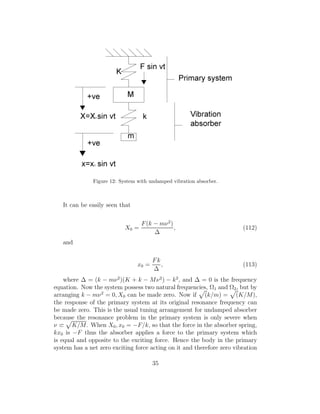
![amplitude. If correctly tuned ω2
= K/M = k/m, and if the mass ratio
µ = m/M, the frequency equation ∆ = 0 is ( [21], p.196)
ν
ω
4
− (2 + µ)
ν
ω
2
+ 1 = 0, (114)
hence
Ω1,2
ω
= 1 +
µ
2
± µ +
µ2
4
1/2
. (115)
For a small µ, Ω1 and Ω2 are very close to each other, and near to ω,
increasing µ gives better separation between Ω1 and Ω2. This is of impor-
tance in systems where the excitation frequency may vary e.g. µ is small,
resonances at Ω1 or Ω2 may be excited. Now:
Ω1
ω
2
= 1 +
µ
2
− µ +
µ2
4
(116)
and
Ω2
ω
2
= 1 +
µ
2
+ µ +
µ2
4
(117)
then multiplying gives
Ω1Ω2 = ω2
(118)
and
Ω1
ω
2
+
Ω2
ω
2
= 2 + µ. (119)
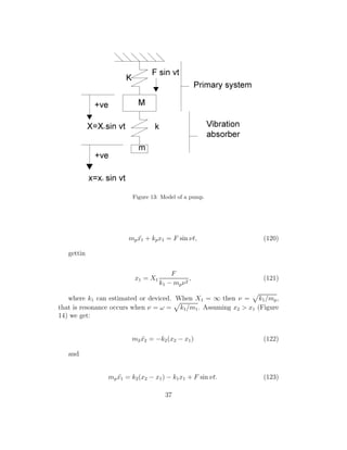
One can use these relations to desing an absorber, and can be used for
instance for a pump having mass of mp rotating at constant speed of ωp
rev/min, giving large unbalance vibrations. Fitting an undamped absorber
so that the natural frequency of the system is removed by 20%. We model
the pump as in Figure 13, so we get the equation of motion:
36](https://image.slidesharecdn.com/dippat-130510045604-phpapp01/85/Master-Thesis-on-Rotating-Cryostats-and-FFT-DRAFT-VERSION-38-320.jpg)
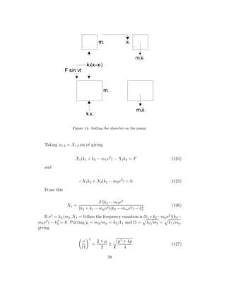
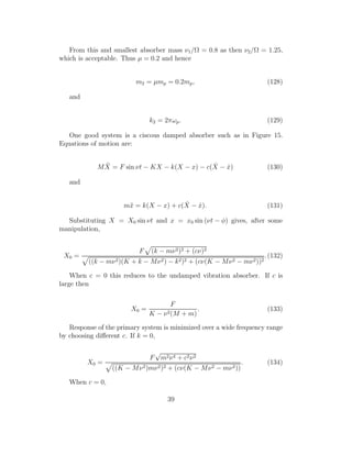
![Figure 15: System with damped vibration absorber.
X0 =
F
K − Mν2
, (135)
and when c is very large,
X0 =
F
K − (M + m)ν2
. (136)
7 Torsional vibrations
Historically torsional modes in machinery were always the first to consider
and analyze, in order to avoid extreme stresses. Today torsional vibration
analysis is routinely done throughout design of rotating machines. Their ex-
istence can be discovered when using dedicated instruments [27] to measure
torsional vibrations. Torsional vibration is an oscillatory angular motion
causing twisting in the shaft of a system. Motion is rarely a concern with
torsional vibration unless it affects the function of a system. It is stresses
that affect the structural integrity and life of components and thus determine
40](https://image.slidesharecdn.com/dippat-130510045604-phpapp01/85/Master-Thesis-on-Rotating-Cryostats-and-FFT-DRAFT-VERSION-42-320.jpg)
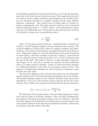
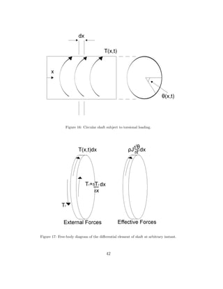
![Consider
δ2
θ
δx2
=
δ2
θ
δt2
. (147)
Let us look at some cases to analyse the cryostat with the above analysis.
Firstly let us make x the length of the cryostat a unilength so that free
end is x = 1 and taking the fixed end at x = 0. The boundary condition
is θ(0, t) = 0, and ˙θ(1, t) = 0 (the derivate is in terms of x). Applying a
moment M is statically applied to the end of the shaft leading to the initial
condition θ(x, 0) = Mx/(JG) = γx. Since the shaft is released from rest
a second initial condition is ˙θ(x, 0) = 0 (the derivative is in terms of t). A
separation of variables is assumed θ(x, t) = X(x)T(t), which gives
1
X(x)
d2
X
dx2
=
1
T(t)
d2
T
dt2
. (148)
leading to
d2
T
dt2
+ λT = 0, (149)
and
d2
X
dx2
+ λX = 0, (150)
where λ is the separation constant. The solution is
T(t) = A cos
√
λt + B sin
√
λt, (151)
where A and B are arbitrary constants of integration. Similarly
T(t) = C cos
√
λx + D sin
√
λx (152)
The initial conditions give C = 0, B = 0 and the only reasonable solution
λk = [(2k − 1)
π
2
]2
k = 1, 2, . . . (153)
44](https://image.slidesharecdn.com/dippat-130510045604-phpapp01/85/Master-Thesis-on-Rotating-Cryostats-and-FFT-DRAFT-VERSION-46-320.jpg)
![Now infinity of solutions arise corresponding to
Xk(x) = Dk sin (2k − 1)
π
2
x (154)
for any Dk. The modes are orthogonal giving
(Xk(x), Xj(x)) =
1
0
DjDk sin (2k − 1)
π
2
x sin (2j − 1)
π
2
xdx = 0 (155)
for j = k, but when k = j we get
1 = (Xk, Xk) =
D2
k
2
(156)
leading to
θ(x, t) =
∞
k=1
√
2 sin (2k − 1)
π
2
x[Ak cos (2k − 1)
π
2
t]. (157)
From the initial conditions we get the last
Ak =
4γ
√
2(−1)k+1
π2(2k − 1)2
(158)
yielding in total
θ(x, t) =
8γ
π2
∞
k=1
(−1)k+1 1
(2k − 1)2
sin((2k − 1)
π
2
x) cos((2k − 1)
π
2
t). (159)
Let us now consider a circular shaft fixed at x = 0 and has a thin disk
of mass moment of inertia I, similar to the electronics above the cryosta,
attached at x = 1. The partial differential equation governing [28]
δθ(1, t)
δx
= −β
δ2
θ(1, t)
δt2
(160)
where β = I/(ρJL). Separation of variables give:
45](https://image.slidesharecdn.com/dippat-130510045604-phpapp01/85/Master-Thesis-on-Rotating-Cryostats-and-FFT-DRAFT-VERSION-47-320.jpg)
![8 Balancing rotation
The unbalance of rotating machinery is the most common malfunction, even
so that any lateral vibrations are usually wrongly thought to be due to un-
balances. In our case the unbalance of the cryostat is obvious as the electric
devices, and pumping systems mounted are not symmetric, and there are
restrictions in placing them. Quite frequently, balancing procedures per-
formed on the machine, which another type of malfunction, worsens the
situation. These unbalances have been recognized for over 100 years. Bal-
ancing procedures are equally old. However during the last 25 years they
have experienced substantial improvements due to implementation of vibra-
tion measuring electronic instruments and application of computers for data
acquisition and processing. For over a century researchers have published
hundreds of papers on how to balance machines. For more advanced methods
one should consult [29]. The problem due to unbalance is easiest to identify
and correct. The unbalance causes vibrations and alternating or variable
stress in the cryostat it self and the supporting structure elements. These
vibrations are directly linked to heat leak, and thus again should be minized
as possible. The balancing problem is solved by either, relocating electronic
equipment or adding masses. After proper balancing, rotating vibrations
should be reduced in the entire range of rotational speeds, including the op-
timal operating speeds, as well as the resonance speed range. The latter is
especially important when the cryostat is operated in hihg speeds exceed-
ing the first, the second, or even higher natural modes of resocance. As the
unbalance force is proportional to the rotational frequency squared [30], the
unbalance-related grows considerably with increasing rotational speed. The
plane that is rigidly attached on the cryostat carrying the electronics can be
thought of as beign a symmetric rotor with the axis of rotation directly in
the middle. The unblance condition changes the rotor mass centerline not to
coincide with the axis of rotation. Unbalance is due to the restricted placing
of the electronic devices mounted on the plane. During rotation, the rotor
unbalance generates a centrifugal force perpendicular to the axis of rotation.
This force excites, rotor lateral vibration e.g. rotor fundamental response.
In the following presentation, the modal approach to the rotor system as a
mechanical structure, has been adopted. At the beginning, the first lateral
mode of the rotor is considered only. The lateral mode can either be rotor
bending mode or susceptibility mode. Conventionally fundamental the vibra-
tion response of the rotor at its lateral mode is due to the inertial centrifugal
exciting force, generated by unbalance. In the modal approach, limited to
the first lateral mode, the unbalance-retaled exciting force is discrete, i.e. an
average integral, lumped effect of the axially distributed unbalance in the
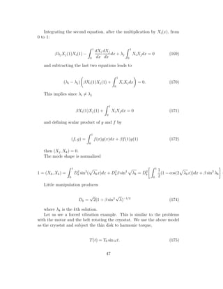
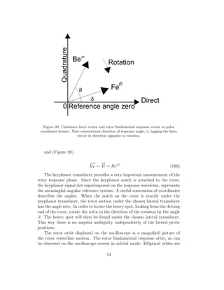
49](https://image.slidesharecdn.com/dippat-130510045604-phpapp01/85/Master-Thesis-on-Rotating-Cryostats-and-FFT-DRAFT-VERSION-51-320.jpg)
![first mode. The average unbalance angular force location will be referred
to as a heavy spot. Rotors are usually similarly constrained in all lateral
directions. Therefore, they exhibit lateral vibrations in space, with two in-
separable components of motion at each specific axial section of the rotor.
These two components result in a two-dimensional orbiting motion of each
axial section. Typically, two displacement proximity transducers, mounted in
XY orthogonal configuration, will measure the lateral vibrations of the rotor
in one axial section plane. The isotropic rotor lateral synchronous motion,
as seen by the displacement transducers 90 degrees apart, will differ by 90
degrees phase angle. The rotor lateral vibrations can be observed on an oscil-
loscope in the time-base mode, and in orbital mode. The latter represents a
magnified image of the actual rotor centerline path in this section. Figure 18
illustrates the waveforms and an orbit of a slightly anisotropic rotor funda-
mental response. The angular position of the force and response vectors are
vital parameters for the balancing procedure. In practical applications, the
response phase is measured by the Keyphasor transducer ( [31], and [32]).
Keyphasor is a transducer generating a signal used in rotating for observing
a once-per-revolution event. A notch is made on the rotor, which during
rotor rotation causes the Keyphasor displacement transducer to produce an
output impulse, every time the Keyphasor notch passes under the trans-
ducer. The one-per-turn impulse signal is simultaneously received, together
with the signals from the rotor lateral displacement-observing transducers.
The Keyphasor signal is usually superimposed on the rotor lateral vibration
response time-base waveform presentation and on rotor orbits. On the os-
cilloscope display, the Keyphasor pulse is connected to the beam intensity
input (the z-axis of the oscilloscope; while the screen displays x and y axis).
The Keyphasor pulse causes modulation of the beam intensity, displaying
a bright dot, followed by a blank spot on the time-base and/or orbit plots.
The sequence bright/blank may vary for different oscilloscopes and for rotor
notch/projection routine, but is always consistent and constant for a partic-
ular oscilloscope and rotor configuration; this sequence should be checked on
rotor waveform time-base responses when the oscilloscope is first used.
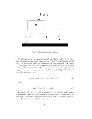
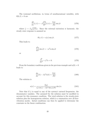
The unbalance force at a constant rotational speed, Ω as seen in Figure
19 can be characterized in the following way. There’s a fixed relation to the
rotating system. The nature of the rotating period is strictly harmonic time-
base, expressed by sin Ωt, cos Ωt or eiΩt
, where t is time. When the frequency
is equal to the actual rotational speed the unbalance is rotating at the same
rate in sync with the rotor rotation. The force F is proportional to three
physical parameters namely: unbalance average, modal mass m, and square
of the rotational speed.
50](https://image.slidesharecdn.com/dippat-130510045604-phpapp01/85/Master-Thesis-on-Rotating-Cryostats-and-FFT-DRAFT-VERSION-52-320.jpg)
![F = mrΩ2
(182)
Force phase that is the angular orientation δ mesured in degrees or radians
from a reference angle zero marked on the rotor circumference. The unbal-
ance force causes rotor response in a form of two-dimensional orbital motion.
The harmonic time-base is expressed by a similar harmonic function as the
unbalance force and the frequency is equal to the actual rotational speed
Ω. Amplitude B is directly proportional to the amplitude of the unbalance
force, and F is inversely proportional to the rotor synchronous dynamic stiff-
ness [33]. Phase lag β represents the angle between the unbalance force vector
and response vector plus the original force phase, δ. The response always lags
the force, thus the phase moves in the direction opposite to rotation. Both
unbalance force and rotor response are characterized by the single frequency
equal to the frequency of the rotational motion. The vibrational signal read
by a pair of XY displacement transducers should, therefore, be filtered to
frequency Ω, or what is the same, to frequency describing synchronous fre-
quency of the rotor response as a multiple of one. There may exist other
frequency components in the rotor response. These possible components of
the vibrational signals are not directly useful for rotor balancing. A vector
filter can, for instance, be used for filtering of the measured signal to the first
component only. In the characterization of both the force and response, the
amplitude and phase were emphasized as two equally important parameters.
Using the complex number formalism, these two parameters can be lumped
into one the force vector and response vector correspondingly. The amplitude
will represent the length of the vector, the phase its angular orientation in
the polar plot, coordinate format. The unbalance force and rotor response
are therefore, described in a very simple way. Unbalance force is:
Fei(Ωt+δ)
= mrΩ2
ei(Ωt+δ)
(183)
and rotor fundamental response
RF = Bei(Ωt+β)
. (184)
The corresponding vectors are obtained when the periodic function of
time, eiΩt
is eliminated:
−→
F = Feiδ
= mrΩ2
ejδ
(185)
53](https://image.slidesharecdn.com/dippat-130510045604-phpapp01/85/Master-Thesis-on-Rotating-Cryostats-and-FFT-DRAFT-VERSION-55-320.jpg)
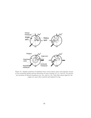
![due to anisotropy of the rotor support system, which is the most common
case in machinery. One Keyphasor dot on the orbit is at a constant posi-
tion, when the rotational speed is constant. It means that during its one
rotation cycle the rotor makes exactly one lateral vibration orbiting cycle.
Direction of orbiting is the same as direction of rotation called forward or-
biting. For a constant rotational speed, the orbit exhibits a stable shape
and the Keyphasor dot appears on the orbit at the same constant angular
position. The phase of the rotor fundamental response is often referred to
as the high spot. It corresponds to the location, on the rotor circumference,
which experiences the largest deflections and stretching deformations at a
specific rotational speed. Although just One-plane balancing does not have
many practical applications in machinery, it provides a meaningful general
scheme for balancing procedures. Basic equation for one plane balancing of
the rotor at any rotational speed is represented by the one mode isotropic
rotor relationship between input force vector, Feiδ
, rotor response vector,
Beiβ
and complex dynamic stiffness [34],
−→
k (Ω):
−→
k (Ω)Beiβ
= Feiδ
(187)
where
−→
k (Ω) = K − MΩ2
+ iDSΩ. (188)
The complex dynamic Stiffness represents a vector with the direct part,
kD = K − MΩ2
and quadrature part kQ = DΩ.
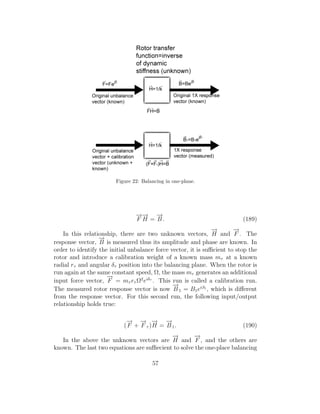
The rotor in Figure 18 is now defined more precisely it contains the rotor
Transfer Function [35], which is an inverse matrix of the Complex Dynamic
Stiffness,
−→
k . The inverse of the complex dynamic dtiffness is also known
receptance. The objective of balancing is to introduce to the rotor a corrective
weight of mass, mc, which would create the inertia centrifugal force vector
equal in magnitude and opposite in phase to the initial unbalance force vector.
This way, the rotor input theoretically becomes nullified and the vibrational
output results also as a zero. In practical balancing procedures, the input
vector force of the initial unbalance has therefore to be identified. Using
again the block diagram formalism, the one-plane balancing at a constant
rotational speed is illustrated in Figure 22.
Introduce the vectorial notation:
−→
F = Feiδ
and
−→
B = Beiβ
, for the
unbalance force vector and response respectively, as well as,
−→
H = 1/
−→
k for
the rotor transfer function vector. The original unbalance response at a
constant speed, Ω is:
55](https://image.slidesharecdn.com/dippat-130510045604-phpapp01/85/Master-Thesis-on-Rotating-Cryostats-and-FFT-DRAFT-VERSION-57-320.jpg)
![done with all the cryostat’s electronics in place, and other set of measure-
ments were done when all the electronics were removed. The measurements
were done in the same way as previous vibrational noise measurements [36].
The measurements were done in the normal, and tangential directions from
the axis of rotation. The rotation speeds were 250, 1000, 2000, 3000 mrad/s.
The accelerometer used is a Bruel and Kjaer Accelerometer Type 4370 [37],
and Bruel and Kjaer preamplifier was used before collecting the data with
Agilent 54641 Oscilloscope [38]. The data aquired was done using TCL, and
transferred by GPIB.
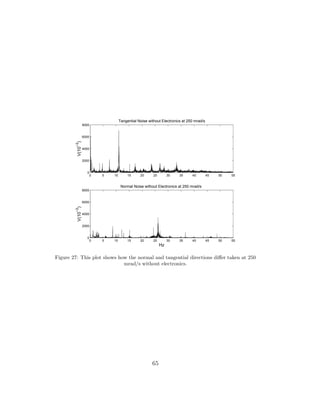
The results were similar to previously done measurements [36]. The nois-
iest direction by far was the tangent of the rotation vector, this means that
the noise was rather torsional rather than back and forth swaying of the
cryostat. The 250 mrad/s speed is a problematic speed as it showed some
risen noise levels. This was propably due that some part of the cryostat
experiences its first harmonic.
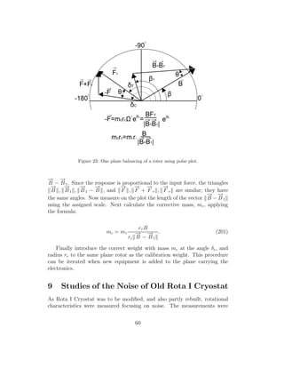
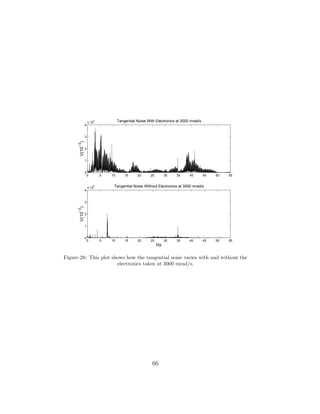
In Figure 24. at 250 mrad/s some peaks in the fourier transform seemed
to be quite visible and large compared to the 1000 mrad/s case. Some of
the peaks have lowered and also disappeared at 1000 mrad/s, but the overall
noise seems to have increased at all frequencies. This is taken with all the
electronics on, and in the tangential direction. In the normal direction the
largest peaks are half to that of tangential and the overall noise is somewhat
lower at all frequencies.
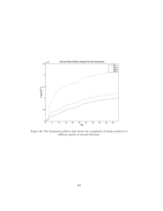
As the speed was increased the noise-levels rose, but not all frequencies
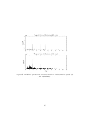
seemed to be affected by this. In Figure 25. the noise-levels are additively
integrated over region up to 55 Hz at different speeds. In this tangential
noise-plot one is able to see the unbalanced increases at different frequencies.
The removal of electronics had an unexpected effect on the noiselevels.
Vibrational noise fell sharply in the measurements after the removal of the
electronics. This was probably due to the fact that load from the air bearings
was lifted, and thus removing some friction. This means that the air bearings
are experiencing their maximum load, and when the electonics are mounted
on the cryostat the friction rises.
The integration without the electronics reveals that the noise at different
speeds in the tangential directions does not vary as expected. Rather the
250 mrad/s case seems to dominate in this situation as can be seen in Figure
28. The moment of inertia has been changed, so the high noise-level at 250
mrad/s is not necessarily a first harmonic that the whole cryostat or the belt
of the rotating motor is experiencing. It could also be that motor is not
functioning perfectly at this speed.
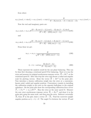
61](https://image.slidesharecdn.com/dippat-130510045604-phpapp01/85/Master-Thesis-on-Rotating-Cryostats-and-FFT-DRAFT-VERSION-63-320.jpg)
![0 5 10 15 20 25 30 35 40 45 50
0
2000
4000
6000
8000
10000
12000
14000
Hz
VHz(10
−3
)
Tangential Additive Noise Integration without Electronics
250
1000
2000
3000
Figure 28: Additive integration is taken without electronics in the tangential direction.
10 Superconducting high-homogeneity mag-
net for NMR measurements
Chemical analysis, and imaging of biological samples are commonly probed
using nuclear magnetic resenance methods. The samples in a magnetic field
are studied using continuous wave NMR causing the samples’s magnetic mo-
ments of the atomic nuclei to arrange in a fashion minimizing the magnetic
potential energy. The NMR frequency of the sample is changed according to
the dependent magnitude, thus the polarization field strenght is sweeped [39]
and the resulting spectrum measured gives information about the structure
Getting a good NMR signal requires the magnetic moments to be as uniform
as possible. A very homogenous field is thus a must, which requires that
the polarizing magnet is constructed with great care. The homogeneity is
defined as the relative deviation from the center point value B0:
|
∆B
B0
| = |
B − B0
B0
|. (202)
One must also take into account the space where the measurements are
to be made. They are in volume very constricted, and the sample as in our
67](https://image.slidesharecdn.com/dippat-130510045604-phpapp01/85/Master-Thesis-on-Rotating-Cryostats-and-FFT-DRAFT-VERSION-69-320.jpg)
![case is helium is to be measured in a cylindrical cell. Solenoid magnet is
thus a very good choice for this experiment, and the field can be represented
in closed form ( [40], [41]). Increasing the coil length and optimizing the
diameter of the solenoid improves the homogeneity, which in general means
decreasing the diameter. The homogeneity is reduces when one moves axially
away from the center, and trying to reduce this short compensation coils at
both ends are placed. The most common of the compensation methods is
the sixth order end compensation [42], in which the correct choice of magnet
dimensions cancels the first five derivative terms in the expansion series of
the field. The homogeneity can also be improved using the Meissner effect,
which occurs as superconducting material is placed in a magnetic field. As
in the case of perfect diamgnet the superconductor sets up surface currents
cancelling the field within the material by opposing magnetization. The
solenoid is surrounded by superconducting material in order to force the
field lines to concentrate in center of the solenoid center [43] and also acts as
a shield for external unwanted fields. The magnet used for the measurements
was already provided [44]. The wire consist of quite fragile Super Con Inc. 18
filament NbTi inside CuNi alloy matrix [45]. As the measurements are done
notably under the critical 4.2 K temperature, there should be no problem of
proper thermalization. The dimensions of the magnet can be seen in Figure
29. The magnet was previously tested merged in liquid helium with maximun
current load of 12.5 A without quenching. The absolute value of the magnetic
field strength for the magnet was not accurately measured as the Hall probe
used by Vesa Lammela was designated to work at temperature range of −10
to 125o
C. The homogeneity of the magnet was therefore to be tested with
actual NMR-measurements.
11 Superconductivity
The phenomenon of superconductivity occurs in specific materials at ex-
tremely low temperatures. The characterization includes exactly zero elec-
trical resistance, and the Meissner effect [46]. The resistivity of the metallic
conductor gradually decreases as temperature is lowered, and drops abruptly
to zero when the material is cooled below the critical temperature. It is a
quantum mechanical phenomenon. The physical properties vary from mate-
rial to material, especially the heat capacity and the critical temperatures.
Regular conductors have a fluid of electrons moving across a heavy ionic
lattice, where the electrons constantly collide with the ions, thus dissipat-
ing phonon energy to the lattice converting into heat. The superconductor
situation differs in that the electronic fluid cannot be distinguished into in-
68](https://image.slidesharecdn.com/dippat-130510045604-phpapp01/85/Master-Thesis-on-Rotating-Cryostats-and-FFT-DRAFT-VERSION-70-320.jpg)
![Figure 29: Number of turns on each layer, and the dimensions of the magnet.
dividual electrons, but it consists of Cooper pairs [47] caused by electrons
exchanging phonons. The Cooper pair fluid energy spectrum possesses an
energy gap amounting to a minimum energy ∆E that is needed to excite the
fluid. When ∆E is larger than the lattice thermal energy kT, there will be
no scattering by the lattice as the Cooper pari fluid is a superfluid without
phonon dissipation. The critical temperature Tc varies with the material,
and convetionally are in the range of 20K to less than 1K. The transition to
superconductivity is accompanied by changes in various physical properties.
In the normal regime the heat capacity is proportional to the temperature,
but at the transition it suffers a discontinous jump, and linearity is impaired.
At the low temperature range it varies as e−α/T
where α is some constant
varying with the material. The transition as indicated by experimental data
is of second-order, but the recent theretical improvements (which are ongo-
ing) show that within the type II regime transition is of second order and
within the type I regime first order, and the two regions are separated by a
tricritical point [48]. Considering the Gibbs free energy per unit volume g,
which is related to internal energy per unit volume u and entropy s:
g = u − Ts (203)
69](https://image.slidesharecdn.com/dippat-130510045604-phpapp01/85/Master-Thesis-on-Rotating-Cryostats-and-FFT-DRAFT-VERSION-71-320.jpg)
![where the volume term has been neglected. The associated magnetic
energy in the presence of an applied magnetic field ¯Ba is − ¯M ·d ¯Ba, where ¯M
is the magnetic dipole moment per unit volume. A change in the free energy
is given by
dg = − ¯M · d ¯Ba − sdT. (204)
Integrating yields:
g(Ba, T) = g(0, T) −
Ba
0
¯M · d ¯Ba. (205)
For type-I-superconductor ¯M = − ¯H [50] due to the Meisness effect, and
thus the previous can be written as:
gS(Ba, T) = gS(0, T) +
Ba
0
BadBa
µ0
= gS(0, T) +
B2
a
2µ0
. (206)
We see B2
a/2µ0 as the extra magnetic energy stored in the field as resulting
from the exclusion from the superconductor. At the transition between the
superconductivity and normal state we have gS(Bc, T) = gN (0, T), where
Bc is the critical magnetic field and the magnetization of the normal state
has been neglected. The entropy difference ∆s < 0 between normal and
superconducting states can be obtained from this using s = −(δg)/δT. Now
the heat capacity per unit volume c = Tδs/δT is:
∆c =
T
µ0
Bc
d2
Bc
dT2
+
dBc
dT
2
, (207)
which shows that there is a discontinuous jump in ∆c even for Bc = 0.
As our superconducting filament behaves as convetional superconductiv-
ity the pairing can be explained by the microscopic BCS theory. The assump-
tion of the BSC theory [49] is from the assupmtion that electrons have some
attration between them overcoming the Coulomb repulsion. This attraction
in most materials is brought indirectly by the interaction between the elec-
trons and the vibrating crystal lattice as the opposite spins becoming paired.
As electron moves through a conductor nearby a positive lattice point causes
another electron with opposite spin to move into the region of higher positive
charge density held together by binding energy Eb. When Eb is higher than
70](https://image.slidesharecdn.com/dippat-130510045604-phpapp01/85/Master-Thesis-on-Rotating-Cryostats-and-FFT-DRAFT-VERSION-72-320.jpg)
![phonon energy from oscillating atoms in the lattice, then the electron pair
will stick together, thus not experiencing resistance and describing an s-wave
superconducting state. Let us look more closely to the electron-phonon in-
teraction. Electron in a crystal with wavevector ¯k1 scatters to ¯k′
1 emitting a
phonon ¯q. Then this phonon is absorbed by a second electron ¯k2 to ¯k′
2 hence
the conservation of crystal momentum:
k1 + k2 = k′
1 + k′
2 = k0. (208)
States in the ¯k-space can interact, but are restricted by the Pauli exclusion
principle corresponding to electron energies between EF and EF + ωD, where
EF is the Fermi energy and ωD is the Debye frequency. The number of allowed
states occur when ¯k1 = −¯k2, and they are called the Cooper pairs [51]. The
transition temperature Tc is given by BSC model [52]
kBTc = 1.14 ωDe−1/V0g(EF )
, (209)
where V0 is the phonon-electron interaction strenght. In the BCS ground
state (T = 0), there is a binding energy 2∆ to the first allowed one-electron
state, in which the Cooper pairing is broken. The gap energy in conventional
superconductors are in the range of 0.2-3 meV, thus very much smaller than
EF . Next we will consider quenching mechanisms for the breaking up of the
superconducting state to normal state. It is exactly this that the Cooper
pairing is broken as some disturbance overcomes this binding energy.
12 Superconductor quenching
We will deal with the matter of quenching here, as it will be quite a impor-
tant factor affecting the work. Quenching occurs when a superconductive
filament goes to normal resistive state. There are three critical parameters
namely temperature, current density, and magnetic field affecting this behav-
ior. When one of these parameters’ critical value 1is exceeded by some phys-
ical process, superconductor becomes normal-conducting. When the cooling
power for the filament is not sufficient the zone of the normal conductor ex-
pands. Usually in a quench case the entire energy stored in the magnet is
dissipated as heat, even burning the filament. There are two main distur-
bances namaley transient and continuous, which can be again divided into
two more causes point and distributed. In the case of continuous disturbance
the steady power becomes a problem due to e.g. bad joint, or soldering. The
71](https://image.slidesharecdn.com/dippat-130510045604-phpapp01/85/Master-Thesis-on-Rotating-Cryostats-and-FFT-DRAFT-VERSION-73-320.jpg)
![distributed disturbances are usually caused by heat leak to the cryogenic
environment. Now transient disturbances are sudden, and can be for exam-
ple caused by a breaking of a turn in a magnet due to excess Lorenz force
moving the turn by δ. In this case the work done by the magnetic field is
BJδ, where J is the current density, and this energy will heat the magnet to
normal state. Our filament is embedded in a copper matrix, which is a good
absorber and distributor of heat, thus if the copper gets good enough contact
where to dissipate the energy, the magnet can stay in superconducting state
even thought some problems persist. For example cooling of the filament by
helium is given by the adiabatic heat balance equation [53]:
ρcu(T(x, t))
I(t)2
Acu(x)
= c(T(x, t))A(x)
dT(x, t)
dt
, (210)
where ρcu is the resistivity of copper, Acu is the copper cross-section of
the composite, I is the current in the filament, T is the temperature of the
filament, and c is the heat capacity. Voltage V (t) is a function of time in the
magnet coil
V (t) = I(t)R(t) + L(I)
dI(t)
dt
−
i
Mi
dI
dt
− UP C, (211)
where I(t) is the current, R(t) is the resistance, L(I) is the self inductance,
Mi is the mutual induction of a neighboring turn or coil, and Upc is the voltage
of the power converter. Now with a good power converter, the quenching
voltage can be given:
VQt) = I(t)R(t) + LQ(t)
dI
dt
, (212)
where LQ is the partial inductance and R(t) is the resistance of the
quenching zone. Taking mutual inductance zero, we get [54]:
VQ(t) = I(t)R(t)(1 − LQ(t)/L). (213)
The quench zone thus expands as resistance and partial inductance grow.
A good power supply can detect this, and switches itself off.
72](https://image.slidesharecdn.com/dippat-130510045604-phpapp01/85/Master-Thesis-on-Rotating-Cryostats-and-FFT-DRAFT-VERSION-74-320.jpg)
![13 Nuclear Magnetic Resonance, and Imag-
ing
Quantum mechanical magnetic proterties of atom’s nucleus can be studied
with the nuclear magnetic resonance (NMR). The pehomenon was first dis-
covered by Isidor Rabi in 1938 [?]. Neutrons and protons have spin, and the
overall spin is determined by the spin quantum number I, and non-zero spin
associates with a non-zero magnetic moment µ by
µ = γI, (214)
where, γ, is the gyromagnetic ratio. Angular momentum quantization,
and orientation is also quantized. The associated quantum number is known
as the magnetic quantum number m, and can only have values from integral
steps of I to −I thus there are 2I + 1 angular momentum states. Taking the
z component Iz:
Iz = m . (215)
The z-component of the magnetic moment is
µz = γIz = mγ . (216)
¯I2
has eigenvalues I that are either integer or half integer. This can be
meaning
(Im µx′ Im′
) = γ (Im Ix′ Im′
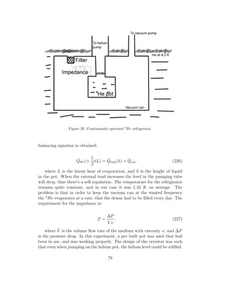
), (217)
where µx′ and Ix′ are components of the operators ¯µ and ¯I along the
arbitrary x′
-direction. This is based on the Wigner-Eckart equation [56]. For
simplicity we consider system of two m states +1/2 and −1/2 by numbers N+
and N−, where the total number N of spins is constant. With the propability
for transition W the absorption of energy is given:
dE
dt
= N+W ω − NW ω = ωWn, (218)
where ω is the angular frequency of the time dependent interaction (or
the frequency of an alternating field driving the transitions), and n has to be
73](https://image.slidesharecdn.com/dippat-130510045604-phpapp01/85/Master-Thesis-on-Rotating-Cryostats-and-FFT-DRAFT-VERSION-75-320.jpg)
![zero for a net absorption. Now in a similar fashion using a alternating field
we get for the absorption energy [57]
dE
dt
= n ωW = n0 ω
W
1 + 2WT1
(219)
where T1 is the spin-lattice relaxation time, and as long as 2WT1 ≪
1 we can increase the power absorbed by increasing the amplitude of the
alternating field. Taking the alternating magnetic field as Hx(t) = Hx0 cos ωt,
and it can be broken into two rotating components with amplitude H1 in
opposite directions. They are denoted by:
¯Hr = H1(¯i cos ωt + ¯j sin tωt) (220)
and
¯HL = H1(¯i cos ωt − ¯j sin ωt). (221)
We consider only ¯HR as ¯HL is just same with negative ω. Taking ωz as
component of ω along z-axis:
¯H1 = H1(¯i cos ωzt + ¯j sin ωzt). (222)
Now the equation of motion with the static field ¯H0 = ¯kH0 is
d¯µ
dt
= ¯µ × γ[ ¯H0 + ¯H1(t)]. (223)
Now moving to a coordinate system such that the system rotates about
the z-direction at frequency ωz then:
δ¯µ
δt
= ¯µ × [¯k(ωz + γH0) +¯iγH1]. (224)
Now near resonance ωz + γH0 ≃ and by setting ωz = −ω states that in
the rotating frame moment acts as though it experiences a static magnetic
field:
¯Heff = ¯k(H0 −
ω
γ
) + H1
¯i. (225)
74](https://image.slidesharecdn.com/dippat-130510045604-phpapp01/85/Master-Thesis-on-Rotating-Cryostats-and-FFT-DRAFT-VERSION-76-320.jpg)
![The effective field exactly when the resonance condition is fullfilled the
effective field is ¯iH1, and a magnetic moment parallel to the static field will
then precess in the y − z plane. Turning H1 on for a wave train of duration
tw so that moment precesses through an agle θ = γH1tw = π so inverting the
moment. Now if θ = π/2 the magnetic moment is turned from z-direction to
the y-direction. Turning H1 off then would make the moment remain at rest
in the rotating frame. Simple method for observing magnetic resonance can
be done with these remarks. Putting a sample in a coil, the axis of which
is perpendicular to ¯H0. Alternating field applied to the coil produces an
alternating magnetic field. Adjusting tw and H1 we can apply a π/2 pulse,
after which the excess magnetization will be perpendicular to ¯H0 precessing
at angular frequency γH0. Now the moments make alternating flux through
the coil inducing emf that may be observed. Now variations of the similar
principle can be used to make measurements using NMR. The method in
our experiment is using continuous wave method. The receiver coils are set
perpendicular to the magnetic field from the magnet. The current is sweeped
in the magnet, and the resonance signal should pick-up in our coil. The
magnitude of nmr resonace signals is proportional to the molar concentration
of the sample [58].
In our experiment the magnet is placed within a vacuum, and in the
middle of the magnet one places the sample to be measured with the pick-up
coils in perpendicular direction to the magnetic field (Figure 30)
The resonance circuit in Figure 30 is tuned for both excitation and de-
tection. At first there was no cooled preamplifier in the setup. The lock-in
amplifier measured the signal from the pick-up coils, which was locked to the
frequency of the oscillator. The oscillator was used to drive the excitation
frequency of the circuit. The magnet was supposed to be swept across to
observe NMR spectrum from the 3
He sample inside the magnet. The test-
ing was supposed to be done for 25 turns per each pick-up coil, and then
50 turns. The pick-up coils were very carefully coiled on glass piece that fit
directly on the sample tube right in the middle. The sample was place in
the center of the magnet, and thus the magnetic field from the magnet and
the pick-up coils were perpendicular. The gyromagnetic ratio of 3
He is 32.43
MHz/T [?]
14 Cooling of the Cryostat
The main purpose in our measurement is to measure the homogeneity of
the superconducting magnet, by doing NMR measurements of normal liquid
3
He, which requires temperatures below 3.19 K. The experiment is done
75](https://image.slidesharecdn.com/dippat-130510045604-phpapp01/85/Master-Thesis-on-Rotating-Cryostats-and-FFT-DRAFT-VERSION-77-320.jpg)
![Figure 30: The setup of the NMR-measurement in our experiment.
in an insulated dewar, see Figure 30. The precooling is done using liquid
nitrogen, which boils at 77 K [59], and liquid N2 has about 60 times the
latent of heat evaporation to that of cryo-helium [60]. Liquid nitrogen is also
an order cheaper than cryo-helium. One very important property of liquid
nitrogen is that it freezes at 63 K, and this has to be taken into account,
when the next cooling phase is done with liquid 4
He. After all the equipment
is placed within the cryostat, and all the necessary preparations have been
done, liquid nitrogen is pumped into the cryostat using a metal tube. This
is done gradually as the liquid evaporates it creates pressure, and there is a
valve to let excess pressure out, but one does not want the pressure to get
much greater than 1.4 Pa in the cryostat. This is because the cool gas will
freeze the insulating rubber in the valve, thus yielding the insulation useless.
After the nitrogen cooling is over the rest of the nitrogen is pumped out
using a narrow nylon tube reaching the bottom of the cryostat. This is solely
for the purpose that the nitrogen freezes otherwise, and it has a rather large
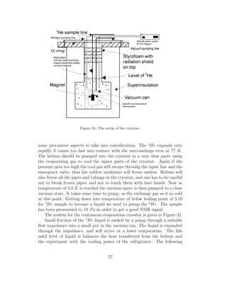
specific heat. The cryostat setup is seen in Figure 31. The vacuum space
at this point is filled with 3
He exchange gas to hasten the cooling of sample
and the magnet. The heat of evaporation for cryo-helium is about 2.6 kJ/l
at its boiling point is 4.2 K. The 4
He used as a cryo-liquid for cooling has
76](https://image.slidesharecdn.com/dippat-130510045604-phpapp01/85/Master-Thesis-on-Rotating-Cryostats-and-FFT-DRAFT-VERSION-78-320.jpg)
![not visible, the repair of the magnet was not possible, and the NMR-studies
could not be completed without the magnet working in the vacuum.
16 Conclusions
The first part of the work consisted of the rotational aspects of Cryo I cryo-
stat. There was a need for very precise rotation [62], and the heat noise was
to be minimized. It was apparent that some of the electronics, were giving
out vibrations at quite precise frequencies. These could be dimished with
the use of dissipating materials and methods suggested, without even that
much work. Also some of the electronics could have their fans relaplaced with
metal spikes as is done in computers, and also let the cooling be done by air
as the cryostat is rotating. This could be a little problematic for some of the
devices. Also some of the pumps gave out vibrations that could diminished
by balacing the pumps with the suggested method. Also the Fourier analysis
was done with data that was not filtered properly, and thus some aliasing
accumulated in the transformed data. This could be avoided by building a
good solid highpass filter according to the Nyquist frequency. The rotation of
the cryostat is done sometimes at quite high speeds, so the balancing of the
cryostat becomes quite important. The electronics could be placed according
to the scheme presented previously, using the one-plane method. Another
way if the electronics cannot be moved around is to place small balancing
weights on the plane carrying the electronics. The balancing method would
require two similar accelerometers, as in this case of this work only one was
available. Also a keyphasor would be needed. In the latter part of the work
a magnet was to be tested for its homogeneity. The problem was apparent
after the meticulous building of the cryostat. The magnet only worked when
it was submerged in 4
He-liquid or 3
He exchange gas. The magnet queched
every time when used in vacuum, and the experiment was thus abandoned,
with the result that the magnet is useless.
References
[1] Emmanuel C. Ifeachor and Barrie W. Jervis, ”Digital Signal Processing:
A Practical Approach”, Addison-Wesley, p. 53 (1993)
[2] Ronald N. Bracewell, The Fourier Transform and Its Applications,
McGraw-Hill, 2000, p. 130.
80](https://image.slidesharecdn.com/dippat-130510045604-phpapp01/85/Master-Thesis-on-Rotating-Cryostats-and-FFT-DRAFT-VERSION-82-320.jpg)
![[3] Bendat, J.S. and Piersol, A.G., Measurement and Analysis of Random
Data, John Wiley, New York, 1966.
[4] Blackman, R. B. and Tukey, J. W., The Measurements of Power Spectra,
Dover, New York, 1956.
[5] Jenkins, G.M. and Watts, D. G., Spectral Analysis and its Applications,
Holden-Day, San Francisco, 1968.
[6] Newland, D. E., An introduction to Random vibrations, spectral and
wavelet analysis, Longman Scientific and Technical, Essex, 1993.
[7] Cooley, J. W., and Tukey, J. W., An Algorithm for the Machine Cal-
culation of Complex Fourier Series, Mathematics of Computation, Vol.
19, 1965, 297-301.
[8] Cooley, J. W., Lewis, P. A. W., and Welch, P. D., Historical Notes on
the Fast Fourier Transform, IEEE Trans. Audio and Electroacoustics,
Vol. AU-15, 1967, No. 2, 76-9
[9] http://www.fftw.org (February, 13, 2008)
[10] Oppenheim, A. V. and R. W. Schafer, Discrete-Time Signal Processing,
Prentice-Hall, 1989, p. 619.
[11] Rader, C. M., ”Discrete Fourier Transforms when the Number of Data
Samples Is Prime,” Proceedings of the IEEE, Vol. 56, June 1968, pp.
1107-1108.
[12] Institute of Electrical and Electronics Engineers Inc. IEEE standard on
piezoelectricity. ANSI/IEEE Std. 176-1987, 1988.
[13] C. R. Fuller, S. J. Elliot, and P. A. Nelson. Active Control of Vibration.
Academic Press, 1996.
[14] Nathan Newman, Considerations in Computing the Useful Frequency
Range of Piezoelectric Accelerometers, NBS Technical Note 487, Na-
tional Bureau of Standards, 1969.
[15] Dranetz, A. I., and Orlacchio, A. W., Chapter 16-Piezoelectric and
Piezoresistive Pickups, Book, Shock and Vibration Handbook, McGraw-
Hill, New York, 1961
[16] Carol F. Vezzetti and Paul S. Lederer, An Experimental Technique for
the Evaluation of Thermal Transient Effects on Piezoelectric Accelerom-
eters, NSB Technical Note 855, National Bureau of Standards, 1975.
81](https://image.slidesharecdn.com/dippat-130510045604-phpapp01/85/Master-Thesis-on-Rotating-Cryostats-and-FFT-DRAFT-VERSION-83-320.jpg)
![[17] Williams, Arthur B. and Taylors, Fred J. Electronic Filter Design Hand-
book, New York: McGraw-Hill, 1988.
[18] Thomas Kugelstadt, Op Amps for Everyone, Chapter 16: Active Filter
Design Techniques, Texas Instruments, 2008
[19] Paul Michael Walmsley, Textures, Vortices and Persistent Currents in a
Slab of 3
He-A,The University of Manchester, 2003
[20] C. F. Beards, Engineering Vibration Analysis with Application to Con-
trol Systems, Edward Arnold, 1995.
[21] C. F. Beards, Structural Vibration Analysis and Damping, Edward
Arnold, New York, 1996.
[22] B. J. Lazan, Damping of Materials and Members in Structural Mechan-
ics, Pergamon, 1968.
[23] Cyril M. Harris, Harris’ Vibration Handbook, Chapters 30-33, New
York: McGraw-Hill, 2002
[24] Paul G. Hoel, Introduction to Mathematical Statistcs, Wiley Publica-
tion, 1966
[25] D. J. Cousins, S. E. May, J. H. Naish, P. M. Wamsley, A. I. Golov,
Design of a Rotating Cryostat to Minimise Vibrational Heating, Dept.
of Physics and Astronomy The Univ. of Manchester, 2003
[26] B. J. Pergamon, Damping of Materials and Members in Structural Mech-
anisms, Pergamon, 1984.
[27] A. Muszynska, Rotordynamics, Chapter 2, Taylor and Frnacis, 2005,
Minden.
[28] S. G. Kelly, Fundamentals of Mechanical Vibrations, Table 9.1, McGraw
Hill, Boston, 2000.
[29] N.F. Rieger, Vibration of Rotating Machinery, Vibration Institute,
Clarendon Hills, IL, 1982
[30] Agnieszka Muszynska, Rotodynamics, Chapter 6. Mechanical Engineer-
ing, The Ohio State University, 2005
[31] http://www.gepower.com/prod_serv/products/oc/en/bently_nevada/acc_vel.htm
8.3.2008
82](https://image.slidesharecdn.com/dippat-130510045604-phpapp01/85/Master-Thesis-on-Rotating-Cryostats-and-FFT-DRAFT-VERSION-84-320.jpg)
![[32] http://www.gepower.com/prod_serv/products/oc/en/downloads/141587.pdf
8.3.2008
[33] http://www.imd.us/pdfs/dynamic-stiffness.pdf
13.3.2008
[34] http://www.bpb-co.com/articles/printableFiles/00understand_stiff_print.pdf
15.3.2008
[35] Ripka J.: Theory of the open end rotor spinning system. In:Rohlena V.
et al: Open-end spinning. Elsevier, Amsterdam 1975.
[36] Aleksanteri Kulvik, ”Vibrational Analysis of Rota I Cryostat”, 2003
[37] http://www.bksv.com/pdf/Bp0196.pdf
July, 31, 2003
[38] http://we.home.agilent.com/cgi-bin/bvpub/agilent/
July, 28, 2003
[39] Ruutu, Ville: NMR experiments on topological defects in 3
He superflu-
ids, Ph.D Thesis, 1996
[40] Lindell, Sihvola: Staattinen kentt¨ateoria. Otatieto, 1995.
[41] J. Vanderlinde, Classical Electromagnetic Theory, Wiley and Sons, New
York, 1993.
[42] Terrell J., Montgomery D.B,: Some Useful Information for the Design
of Air-Core Solenoids, National Magnet Laboratory MIT, 1961
[43] Brehm, J.J. Mullin: Introduction to the Structure of Matter: A Course
in Modern Physics, Wiley, 1989
[44] Vesa Lammela, Superconducting high-homogeneity magnet for low-field
NMR measurements, TKK Materiaalifysiikka, 2001
[45] SW-18 wire by Supercon Inc. 830 Turnpike, Boston Ma. USA
[46] M. Tinkham, Introduction to Superconductivity, 2nd Ed., Dover Books
on Physics (2004)
[47] L.N. Cooper: Bound Electron Pairs in a Degenerate Fermi Gas, Phys.
Rev 104(4), (1189), 1956.
83](https://image.slidesharecdn.com/dippat-130510045604-phpapp01/85/Master-Thesis-on-Rotating-Cryostats-and-FFT-DRAFT-VERSION-85-320.jpg)
![[48] http://en.wikipedia.org/wiki/Superconductivity
13.4.2008
[49] J. Baardeen, L.N. Cooper, and J.R. Schrieffer, Microscopic Theory of
Superconductivity, Phys. Rec. 106, 162-164, 1957
[50] Stephen Elliott, The Physics and Chemistry of Solids, Wiley, 2000, p.
466
[51] Ibach and Luth, Solid State Physics, Springer-Verlag GmbH and Co.
KG, 1995, p. 230-231
[52] [51], p. 245
[53] Surendran Puthiyedath, Quenching and Protection of Superconducting
Magnets for LHC, CERN-INDIA Collaborator, BARC, Mumbai, India,
2005
[54] Martin N. Wilson, Superconducting Magnets; Oxford Science Publica-
tions, 1987
[55] Rabi, I. I., Zacharias, J. R., Millman, S. and Kusch, P. (1938). A New
Method of Measuring Nuclear Magnetic Moment. Physical Review 53,
318-318
[56] C.P. Slichter, Principles of Magnetic Resonance, Springer, 1980, p. 279
[57] [56], p. 9
[58] http://www.cem.msu.edu/~reusch/VirtTxtJml/Spectrpy/nmr/nmr1.htm
13.4.2008
[59] http://en.wikipedia.org/wiki/Liquid_nitrogen
14.4.2008
[60] F. Pobell, Matter and Methods at Low Temperatures, Springer-Verlag
1992. p. 82
[61] E . Ward , L . Hedlund , W . Kurylo , C . Wheeler , G . Cofer , M .
Dewhirst , L . Marks , Z . Vujaskovic; Proton and hyperpolarized helium
magnetic resonance imaging of radiation-induced lung injury in rats1 .
International Journal of Radiation OncologyBiologyPhysics , Volume 58
, Issue 5 , Pages 1562 - 1569
84](https://image.slidesharecdn.com/dippat-130510045604-phpapp01/85/Master-Thesis-on-Rotating-Cryostats-and-FFT-DRAFT-VERSION-86-320.jpg)
![[62] U. Parts, V. M. Ruutu, J. H. Koivuniemi, Yu. M. Bunkov, V. V.
Dmitriev, M. Fogelstr¨om, M. Huebner, Y. Kondo, N. B. Kopnin, J.
S. Korhonen, M. Krusius, O. V. Lounasmaa, P. I. Soininen and G. E.
Volovik; Single-Vortex Nucleation in Rotating Superfluid 3
He−B, LTL
HUT 1995, Espoo
85](https://image.slidesharecdn.com/dippat-130510045604-phpapp01/85/Master-Thesis-on-Rotating-Cryostats-and-FFT-DRAFT-VERSION-87-320.jpg)

This thesis studied the vibrational and rotational aspects of the Cryo I Helsinki cryostat using Fourier analysis methods. Extensive Fourier analysis was performed to model the vibrations mathematically. The goal was to lower noise levels to improve cryostat operations. The second part of the work tested the homogeneity of a superconducting magnet. Significant preparation was required to build testing equipment for evaluating the magnet.


![Circuit Network Analysis - [Chapter3] Fourier Analysis](https://cdn.slidesharecdn.com/ss_thumbnails/ch3-150613063858-lva1-app6891-thumbnail.jpg?width=640&height=640&fit=bounds)