Download to read offline


![Fourier Series of a Periodic FunctionFourier Series of a Periodic Function
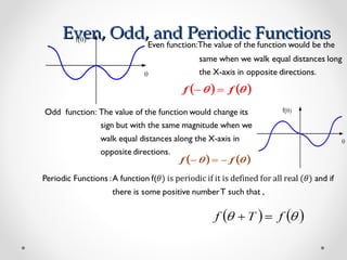
Definition : A Fourier series may be defined as an expansion of a
function in a series of sines and cosines such as ,
0<x<2π
The coefficients are related to the periodic function f(x)
by definite integrals:
Henceforth we assume f satisfies the following (Dirichlet)
conditions:
(1) f(x) is a periodic function;
(2) f(x) has only a finite number of finite discontinuities;
(3) f(x) has only a finite number of extrem values, maxima and
minima in the interval [0,2p].](https://image.slidesharecdn.com/160280102001c1aem-171011170020/85/160280102001-c1-aem-5-320.jpg)

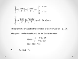


![Fourier IntegralFourier Integral
If f(x) and f’(x) are piecewise continuous in every finite interval, and
f(x) is absolutely integrable on R, i.e.
converges, then
Remark: the above conditions are sufficient, but not necessary.
16
∫ ∫
∞
∞−
∞
∞−
−
=++− dwdttfeexfxf iwtiwx
)(
2
1
)]()([
2
1
π](https://image.slidesharecdn.com/160280102001c1aem-171011170020/85/160280102001-c1-aem-16-320.jpg)

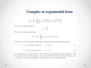


1) Fourier series and integrals are used to represent periodic functions as an infinite sum or integral of sines and cosines. They are useful for solving differential equations. 2) The Fourier series of a periodic function f(x) with period T is the sum of its coefficients multiplied by sines and cosines of integer multiples of x/T. The coefficients are calculated using integrals involving f(x). 3) Half range expansions like half range cosines (HRC) and half range sines (HRS) are used when f(x) is defined on a finite interval, by extending it to a periodic function on the entire real line.