Prof. Rajkumar Teotia 
Institute of Advanced Management and Research (IAMR) 
Address: 9th Km Stone, NH-58, Delhi-Meerut Road, Duhai,Ghaziabad (U.P) 
- 201206 
Ph:0120-2675904/905 Mob:9999052997 Fax: 0120-2679145 
e mail: rajkumarteotia@iamrindia.com
Dispersion measures the extent to which the items vary 
from some central value. It may be noted that the measures 
of dispersion measure only the degree (the amount of 
variation) but not the direction of variation. 
The various measures of central value give us one single 
figure that represents the entire data. But the average alone 
cannot adequately describe a set of observations, unless all 
the observations are the same. It is necessary to describe 
the variability or dispersion of the observations.
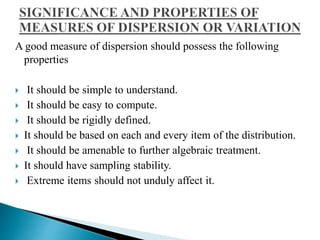
A good measure of dispersion should possess the following 
properties 
 It should be simple to understand. 
 It should be easy to compute. 
 It should be rigidly defined. 
 It should be based on each and every item of the distribution. 
 It should be amenable to further algebraic treatment. 
 It should have sampling stability. 
 Extreme items should not unduly affect it.
 Range 
 Inter-quartile range or Quartile Deviation 
 Mean deviation or Average Deviation 
 Standard Deviation 
 Lorenz curve.
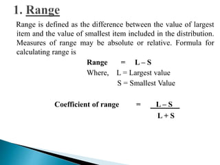
Range is defined as the difference between the value of largest 
item and the value of smallest item included in the distribution. 
Measures of range may be absolute or relative. Formula for 
calculating range is 
Range = L – S 
Where, L = Largest value 
S = Smallest Value 
Coefficient of range = L – S 
L + S
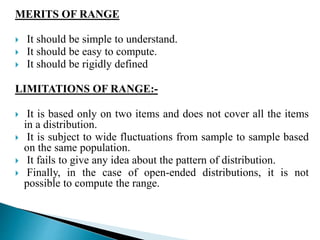
MERITS OF RANGE 
 It should be simple to understand. 
 It should be easy to compute. 
 It should be rigidly defined 
LIMITATIONS OF RANGE:- 
 It is based only on two items and does not cover all the items 
in a distribution. 
 It is subject to wide fluctuations from sample to sample based 
on the same population. 
 It fails to give any idea about the pattern of distribution. 
 Finally, in the case of open-ended distributions, it is not 
possible to compute the range.
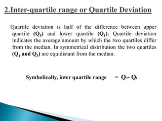
Quartile deviation is half of the difference between upper 
quartile (Q3) and lower quartile (Q1). Quartile deviation 
indicates the average amount by which the two quartiles differ 
from the median. In symmetrical distribution the two quartiles 
(Q1 and Q3) are equidistant from the median. 
Symbolically, inter quartile range = Q3- Ql
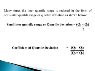
Many times the inter quartile range is reduced in the form of 
semi-inter quartile range or quartile deviation as shown below: 
Semi inter quartile range or Quartile deviation = (Q3 – Ql) 
2 
Coefficient of Quartile Deviation = (Q3 – Ql) 
(Q3 + Ql )
MERITS OF QUARTILE DEVIATION 
The following merits are entertained by quartile deviation: 
 As compared to range, it is considered a superior measure 
of dispersion. 
 In the case of open-ended distribution, it is quite suitable. 
 Since it is not influenced by the extreme values in a 
distribution, it is particularly suitable in highly skewed or 
erratic distributions. 
.
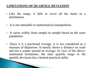
LIMITATIONS OF QUARTILE DEVIATION 
 Like the range, it fails to cover all the items in a 
distribution. 
 It is not amenable to mathematical manipulation. 
 It varies widely from sample to sample based on the same 
population. 
 Since it is a positional average, it is not considered as a 
measure of dispersion. It merely shows a distance on scale 
and not a scatter around an average. In view of the above-mentioned 
limitations, the inter quartile range or the 
quartile deviation has a limited practical utility
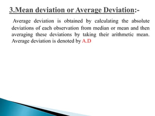
Average deviation is obtained by calculating the absolute 
deviations of each observation from median or mean and then 
averaging these deviations by taking their arithmetic mean. 
Average deviation is denoted by A.D
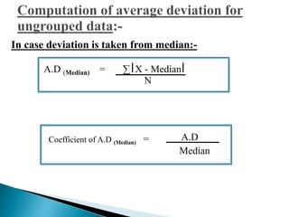
In case deviation is taken from median:- 
A.D (Median) = Σ X - Median 
A.D 
Median 
N 
Coefficient of A.D (Median) =
In case deviation is taken from mean:- 
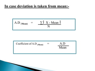
A.D (Mean) = Σ X - Mean 
N 
Coefficient of A.D (Mean) = A.D 
Mean
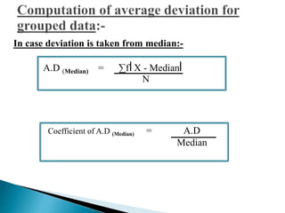
In case deviation is taken from median:- 
A.D (Median) = Σf X - Median 
N 
Coefficient of A.D (Median) = A.D 
Median
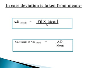
A.D (Mean) = Σf X - Mean 
N 
Coefficient of A.D (Mean) = A.D 
Mean
MERITS OF MEAN DEVIATION 
 A major advantage of mean deviation is that it is simple to 
understand and easy to calculate. 
 It takes into consideration each and every item in the 
distribution. As a result, a change in the value of any item 
will have its effect on the magnitude of mean deviation. 
 The values of extreme items have less effect on the value 
of the mean deviation. 
 As deviations are taken from a central value, it is possible 
to have meaningful comparisons of the formation of 
different distributions.
LIMITATIONS OF MEAN DEVIATION 
 It is not capable of further algebraic treatment. 
 At times it may fail to give accurate results. The mean 
deviation gives best results when deviations are taken from the 
median instead of from the mean. But in a series, which has 
wide variations in the items, median is not a satisfactory 
measure. 
 Strictly on mathematical considerations, the method is wrong 
as it ignores the algebraic signs when the deviations are taken 
from the mean.
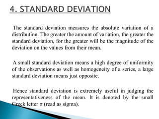
The standard deviation measures the absolute variation of a 
distribution. The greater the amount of variation, the greater the 
standard deviation, for the greater will be the magnitude of the 
deviation on the values from their mean. 
A small standard deviation means a high degree of uniformity 
of the observations as well as homogeneity of a series, a large 
standard deviation means just opposite. 
Hence standard deviation is extremely useful in judging the 
representativeness of the mean. It is denoted by the small 
Greek letter σ (read as sigma).
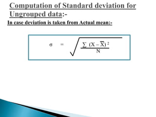
In case deviation is taken from Actual mean:- 
σ = Σ (X – X) 2 
N
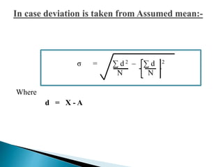
Where 
σ = Σ d 2 – Σ d 2 
d = X - A 
N N
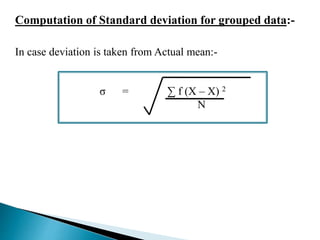
Computation of Standard deviation for grouped data:- 
In case deviation is taken from Actual mean:- 
σ = Σ f (X – X) 2 
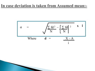
N
σ = Σ fd 2 – Σ fd 2 x i 
Where d = X – A 
i 
N N
Coefficient of variation:- 
Coefficient of variation is calculated by the following formula 
Where, 
C.V = σ x 100 
X 
C.V = coefficient of variation 
σ = standard deviation. 
X = Arithmetic Mean.
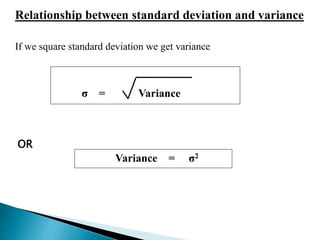
Relationship between standard deviation and variance 
If we square standard deviation we get variance 
OR 
σ = Variance 
Variance = σ2
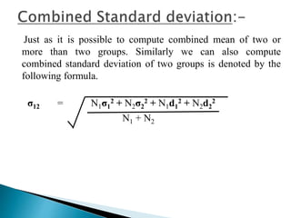
Just as it is possible to compute combined mean of two or 
more than two groups. Similarly we can also compute 
combined standard deviation of two groups is denoted by the 
following formula. 
σ12 = N1σ1 
2 + N2σ2 
2 + N1d1 
2 + N2d2 
2 
N1 + N2
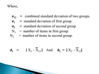
Where, 
σ12 = combined standard deviation of two groups. 
σ1 = standard deviation of first group. 
σ2 = standard deviation of second group 
N1 = number of items in first group. 
N2 = number of items in second group. 
d1 = X1 – X12 And d2 = X2 – X12
PROPERTIES OF THE STANDARD DEVIATION:- 
 The sum of squares of the deviation of all observation from arithmetic mean is 
Minimum. 
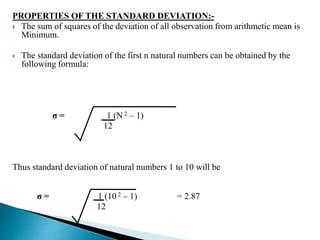
 The standard deviation of the first n natural numbers can be obtained by the 
following formula: 
σ = 1 (N 2 – 1) 
12 
Thus standard deviation of natural numbers 1 to 10 will be 
σ = 1 (10 2 – 1) = 2.87 
12
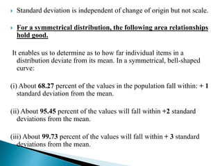
 Standard deviation is independent of change of origin but not scale. 
 For a symmetrical distribution, the following area relationships 
hold good. 
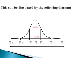
It enables us to determine as to how far individual items in a 
distribution deviate from its mean. In a symmetrical, bell-shaped 
curve: 
(i) About 68.27 percent of the values in the population fall within: + 1 
standard deviation from the mean. 
(ii) About 95.45 percent of the values will fall within +2 standard 
deviations from the mean. 
(iii) About 99.73 percent of the values will fall within + 3 standard 
deviations from the mean.
68.27% 
95.45% 
X - 3σ X - 2σ X - σ X X + σ X + 2σ X - 3σ
This measure of dispersion is graphical. It is known as the 
Lorenz curve named after Dr. Max Lorenz. It is generally used 
to show the extent of concentration of income and wealth. The 
steps involved in plotting the Lorenz curve are: 
 Convert a frequency distribution into a cumulative frequency 
table. 
 On the X – axis, start from 0 to 100 and take the percent of 
variable. 
 On the Y – axis, start from 0 to 100 and take the percent of 
variable.
 Draw a diagonal line joining 0 with 100. This is known as line 
of equal distribution. Any point on this line shows the same 
percent on X as on Y 
 Plot the various points corresponding to X and Y and join 
them. The distribution so obtained, unless it is exactly equal, 
will always curve below the diagonal line. If two curves of 
distribution are shown on the same Lorenz presentation, the 
curve that is farthest from the diagonal line represents the 
greater inequality.
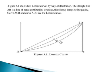
Figure 3.1 shows two Lorenz curves by way of illustration. The straight line 
AB is a line of equal distribution, whereas AEB shows complete inequality. 
Curve ACB and curve ADB are the Lorenz curves