The document discusses various measures used to describe the dispersion or variability in a data set. It defines dispersion as the extent to which values in a distribution differ from the average. Several measures of dispersion are described, including range, interquartile range, mean deviation, and standard deviation. The document also discusses measures of relative standing like percentiles and quartiles, and how they can locate the position of observations within a data set. The learning objectives are to understand how to describe variability, compare distributions, describe relative standing, and understand the shape of distributions using these measures.

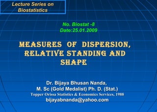
1. Lecture Series on
Biostatistics
No. Biostat -8
Date:25.01.2009
MEASURES OF DISPERSION,
RELATIVE STANDING AND
SHAPE
Dr. Bijaya Bhusan Nanda,
M. Sc (Gold Medalist) Ph. D. (Stat.)
Topper Orissa Statistics & Economics Services, 1988
bijayabnanda@yahoo.com

2. CONTENTS
 What is measures of dispersion?
 Why measures of dispersion?
 How measures of dispersions are calculated?
Range
Quartile deviation or semi inter-quartile range,
Mean deviation and
Standard deviation.
Methods for detecting outlier
 Measure of Relative Standing
 Measure of shape

3. LEARNING OBJECTIVE
 They will be able to:
describe the homogeneity or heterogeneity
of the distribution,
understand the reliability of the mean,
compare the distributions as regards the
variability.
describe the relative standing of the data
and also shape of the distribution.

4. What is measures of dispersion?
(Definition)
Central tendency measures do not
reveal the variability present in the
data.
Dispersion is the scattered ness of
the data series around it average.
Dispersion is the extent to which
values in a distribution differ from the
average of the distribution.

5. Why measures of dispersion?
(Significance)
 Determine the reliability of an
average
 Serve as a basis for the control
of the variability
 To compare the variability of
two or more series and
 Facilitate the use of other
statistical measures.

6. Dispersion Example
 Number of minutes 20  X:Mean Time – 14.6
clients waited to see a
consulting doctor minutes
Consultant Doctor  Y:Mean waiting time
X Y 14.6 minutes
05 15 15 16  What is the difference
12 03 12 18 in the two series?
04 19 15 14
37 11 13 17
06 34 11 15
X: High variability, Less consistency.
Y: Low variability, More Consistency

7. Frequency curve of distribution of
three sets of data
C
A
B

8. Characteristics of an Ideal Measure of
Dispersion
It should be rigidly defined.
1.
It should be easy to understand and easy to calculate.
2.
It should be based on all the observations of the data.
3.
It should be easily subjected to further mathematical
4.
It should be least affected by the sampling fluctuation .
5.
It should not be unduly affected by the extreme values.
6.

9. How dispersions are measured?
 Measure of dispersion:
 Absolute: Measure the dispersion in the
original unit of the data.
 Variability in 2 or more distrn can be
compared provided they are given in the
same unit and have the same average.
 Relative: Measure of dispersion is free from
unit of measurement of data.
 It is the ratio of a measaure of absolute
dispersion to the average, from which
absolute deviations are measured.
 It is called as co-efficient of dispersion.

10. How dispersions are measured? Contd.
 The following measures of
dispersion are used to study the
variation:
 The range
 The inter quartile range and
quartile deviation
 The mean deviation or average
deviation
 The standard deviation

11. How dispersions are measured? Contd.
Range:
The difference between the values of the two
extreme items of a series.
Example:
Age of a sample of 10 subjects from a population
of 169subjects are:
X1 X2 X3 X4 X5 X6 X7 X8 X9 X10
42 28 28 61 31 23 50 34 32 37
The youngest subject in the sample is
23years old and the oldest is 61 years, The
range: R=XL – Xs
= 61-23 =38

12. Co-efficient of Range:
R = (XL - XS) / (XL + XS)
= (61 -23) / (61 + 23) =38 /84 = 0.452
Characteristics of Range
 Simplest and most crude measure of
dispersion
 It is not based on all the observations.
 Unduly affected by the extreme values
and fluctuations of sampling.
 The range may increase with the size of
the set of observations though it can
decrease
 Gives an idea of the variability very
quickly

13. Percentiles, Quartiles (Measure of Relative Standing)
and Interquartile Range
 Descriptive measures that locate the relative position of an
observation in relation to the other observations are called
measures of relative standing.
 They are quartiles, deciles and percentiles
 The quartiles & the median divide the array into four equal parts,
deciles into ten equal groups, and percentiles into one hundred
equal groups.
 Given a set of n observations X1, X2, …. Xn, the pth percentile ‘P’ is the
value of X such that ‘p’ per cent of the observations are less than
and 100 –p per cent of the observations are greater than P.
 25th percentile = 1st Quartile i.e., Q1
 50th percentile = 2nd Quartile i.e., Q2
 75th percentile = 3rd Quartile i.e., Q3

14. QL M QU
Figure 8.1 Locating of lower, mid and upper quartiles

15. Percentiles, Quartiles and Interquartile Range Contd.
n+1
Q1 = th ordered observation
4
Q2 = 2(n+1) th ordered observation
4
Q3 = 3(n+1) th ordered observation
4
Interquartile Range (IQR): The difference
between the 3rd and 1st quartile.
IQR = Q3 – Q1
Semi Interquartile Range:= (Q3 – Q1)/ 2
Coefficient of quartile deviation:
(Q3 – Q1)/(Q3 + Q1)

16. Interquartile Range
Merits:
 It is superior to range as a measure of dispersion.
 A special utility in measuring variation in case of open end
distribution or one which the data may be ranked but measured
quantitatively.
 Useful in erratic or badly skewed distribution.
 The Quartile deviation is not affected by the presence of
extreme values.
Limitations:
 As the value of quartile deviation dose not depend upon every
item of the series it can’t be regarded as a good method of
measuring dispersion.
 It is not capable of mathematical manipulation.
 Its value is very much affected by sampling fluctuation.

17.  Another measure of relative standing is the z-score
for an observation (or standard score).
 It describes how far individual item in a distribution
departs from the mean of the distribution.
 Standard score gives us the number of standard
deviations, a particular observation lies below or above
the mean.
Standard xscore (or z -score) is defined as follows:
z-score=
For a population: X-µ
σ
where X =the observation from the population
µ the population mean, σ = the population s.d
For a sample z-score= X-X
s
where X =the observation from the sample
X the sample mean, s = the sample s.d

18. Mean Absolute Deviation (MAD) or Mean
Deviation (MD)
 The average of difference of the values of items from some average
of the series (ignoring negative sign), i.e. the arithmetic mean of the
absolute differences of the values from their average .
Note:
1. MD is based on all values and hence cannot be calculated for open-
ended distributions.
2. It uses average but ignores signs and hence appears unmethodical.
3. MD is calculated from mean as well as from median for both
ungrouped data using direct method and for continuous
distribution using assumed mean method and short-cut-method.
4. The average used is either the arithmetic mean or median

19. Computation of Mean absolute Deviation
For individual series: X1, X2, ……… Xn
∑ |Xi -X|
M.A.D =
n
For discrete series: X1, X2, ……… Xn & with
corresponding frequency f1, f2, ……… fn
∑ fi |Xi -X|
M.A.D = ∑ fi
X: Mean of the data series.

20. Computation of Mean absolute Deviation:
For continuous grouped data: m1, m2, …… mn are the
class mid points with corresponding class
frequency f1, f2, ……… fn
∑ fi|mi -X|
M.A.D = ∑fi
X: Mean of the data series.
Coeff. Of MAD: = (MAD /Average)
The average from which the Deviations are
calculated. It is a relative measure of dispersion
and is comparable to similar measure of other
series.

21. Example:
Find MAD of Confinement after delivery in the
following series.
Days of No. of Total days of Absolute fi|Xi - X|
Confinement patients (f) confinement of each Deviation
( X) group Xf from mean
|X - X |
6 5 30 1.61 8.05
7 4 28 0.61 2.44
8 4 32 1.61 6.44
9 3 27 2.61 7.83
10 2 20 3.61 7.22
Total 18 137 31.98
X = Mean days of confinement = 137 / 18 = 7.61
MAD=31.98 / 18=1.78, Coeff.of MAD= 1.78/7.61=0.233

22. Problem:
Find the MAD of weight and coefficient of MAD of
470 infants born in a hospital in one year from following
table.
Weight 2.0-2.4 2.5-2.9 3.0-3.4 3.5-3.9 4.0-4.4 4.5+
in Kg
No. of 17 97 187 135 28 6
infant

23. Merits and Limitations of MAD
 Simple to understand and easy to compute.
 Based on all observations.
 MAD is less affected by the extreme items than
the Standard deviation.
 Greatest draw back is that the algebraic signs
are ignored.
 Not amenable to further mathematical
treatment.
 MAD gives us best result when deviation is
taken from median. But median is not
satisfactory for large variability in the data. If
MAD is computed from mode, the value of the
mode can not be determined always.

24. Standard Deviation (σ)
It is the positive square root of the average of squares
of deviations of the observations from the mean. This is
also called root mean squared deviation (σ) .
For individual series: x1, x2, ……… xn
Σ ( xi–x )2 ∑xi2 ∑xi 2
σ=
√ ------------
n
σ=
√ n -( n )
For discrete series: X1, X2, ……… Xn & with
corresponding frequency f1, f2, ……… fn
Σ fi ( xi–x )2
σ= ∑fixi2 ∑fixi 2
------------
Σ fi
σ=
∑fi -( ∑ f )
i

25. Standard Deviation (σ) Contd.
For continuous grouped series with class
midpoints : m1, m2, ……… mn & with
corresponding frequency f1, f2, ……… fn
Σ fi ( mi–x )2
σ= ∑fimi2 ∑fimi 2
√ ------------
Σ fi
σ=
∑ fi -( ∑ f )
i
Variance: It is the square of the s.d
Coefficient of Variation (CV): Corresponding
Relative measure of dispersion.
σ
CV = ------- × 100
X

26. Characteristics of Standard Deviation:
 SD is very satisfactory and most widely used
measure of dispersion
 Amenable for mathematical manipulation
 It is independent of origin, but not of scale
 If SD is small, there is a high probability for
getting a value close to the mean and if it is large,
the value is father away from the mean
 Does not ignore the algebraic signs and it is less
affected by fluctuations of sampling
 SD can be calculated by :
• Direct method
• Assumed mean method.
• Step deviation method.

27.  It is the average of the distances of the observed
values from the mean value for a set of data
 Basic rule --More spread will yield a larger SD
Uses of the standard deviation
 The standard deviation enables us to determine,
with a great deal of accuracy, where the values
of a frequency distribution are located in relation
to the mean.
 Chebyshev’s Theorem
• For any data set with the mean ‘µ’ and the
standard deviation ‘s’ at least 75% of the
values will fall within the 2σ interval and at
least 89% of the values will fall within the 3σ
interval of the mean

28. TABLE: Calculation of the standard deviation (σ)
Weights of 265 male students at the university of Washington
Class-Interval f d fd fd2
(Σƒd2) (Σfd)2
(Weight)
σ= - ×(i)
n n2
90-99 1 -5 -5 25
100-109 1 -4 -4 16 931 (99)2
110-119 9 -3 -27 81 = - ×(10)
265 265
120-129 30 -2 -60 120
130-139 42 -1 -42 42
140-149 66 0 0 0 (3.5132 – 0.1396) (×10)
=
150-159 47 1 47 47
160-169 39 2 78 156 = (1.8367) (10)
170-179 15 3 45 135
180-189 11 4 44 176
= 18.37 or 18.4
d = (Xi –A)/i n = Σfi
190-199 1 5 5 25
200-209 3 6 18 108 . A = 144.5, i = 10
n =265 Σƒd= 99 Σƒd2 = 931

29.  Means, standard deviation, and coefficients of variation of the age
distributions of four groups of mothers who gave birth to one or
more children in the city of minneapol in: 1931 to 1935. Interprete
the data
CLASSIFICATION X σ CV
Resident married 28.2 6.0 21.3
Non-resident married 29.5 6.0 20.3
Resident unmarried 23.4 5.8 24.8
Non-resident unmarried 21.7 3.7 17.1
Example: Suppose that each day laboratory technician A completes
40 analyses with a standard deviation of 5. Technician B completes
160 analyses per day with a standard deviation of 15. Which
employee shows less variability?

30. Uses of Standard deviation
 Uses of the standard deviation
• The standard deviation enables us to
determine, with a great deal of accuracy,
where the values of a frequency
distribution are located in relation to the
mean. We can do this according to a
theorem devised by the Russian
mathematician P.L. Chebyshev (1821-
1894).

31. Measure of Shape
The fourth important numerical characteristic of a
data set is its shape: Skewness and kurtosis.
 Skewness
• Skewness characterizes the degree of
asymmetry of a distribution around its
mean. For a sample data, the
skewness is defined by the formula:
3
n n
 xi − x 
Skewness = ∑ s 
(n − 1)(n − 2) i =1  
where n = the number of observations in the sample,
xi= ith observation in the sample, s= standard deviation of
the sample, x = sample mean

32. Measure of Shape
Figure 8.2 +ve or Right-skewed
distribution

33. Kurtosis:
Kurtosis characterizes the relative peakedness or flatness of
a distribution compared with the bell-shaped distribution
(normal distribution).
Kurtosis of a sample data set is calculated by the formula:

 n(n + 1) n
 xi − x  
4
 3(n − 1) 2
Kurtosis =  ∑  s   − (n − 2)(n − 3)
 (n − 1)(n − 2)(n − 3) i =1   
 
Positive kurtosis indicates a relatively peaked distribution.
Negative kurtosis indicates a relatively flat distribution.

34. The distributions with positive and negative kurtosis
are depicted in Figure 8.4 , where the distribution with
null kurtosis is normal distribution.

35. REFERENCE
1. Mathematical Statistics- S.P Gupta
2. Statistics for management- Richard I.
Levin, David S. Rubin
3. Biostatistics A foundation for Analysis
in the Health Sciences.

36. THANK YOU