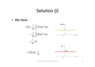
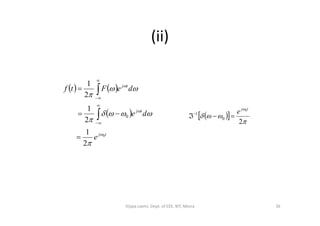
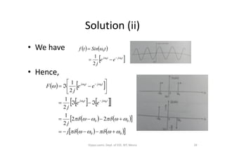
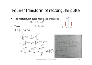
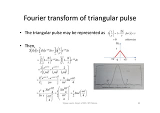
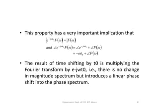
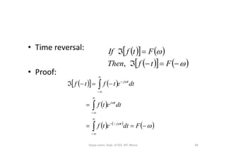
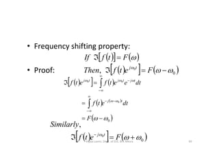
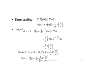
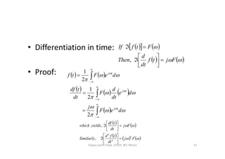
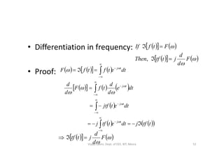
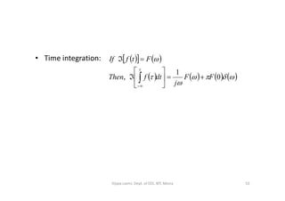
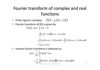
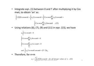
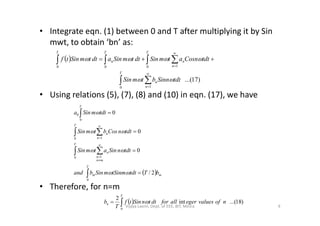
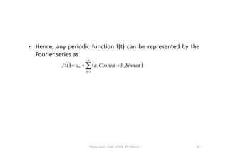
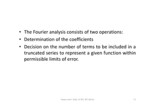
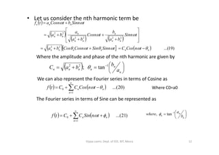
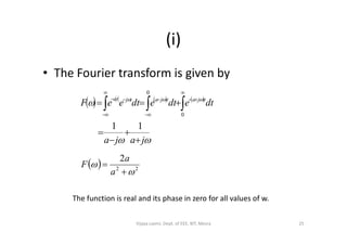
This document discusses the Fourier transform method for analyzing linear systems. It begins by introducing Fourier series as a way to represent periodic functions as an infinite series of sinusoids. It then discusses how the Fourier transform can be used to represent non-periodic functions. The key steps of the Fourier transform method are outlined, including determining the Fourier coefficients, representing signals in the frequency domain, and taking the inverse transform. Properties of Fourier series and examples of periodic and non-periodic signals are also briefly covered. The document provides an overview of the Fourier transform method for analyzing input/output signals of linear networks in both the time and frequency domains.

1. Module III
Fourier Transform MethodFourier Transform Method
By
Dr. Vijaya Laxmi
Dept. of EEE, BIT, Mesra
1Vijaya Laxmi, Dept. of EEE, BIT, Mesra

2. Introduction
• The steady-state response of a linear system to DC
and sinusoidal excitations can be found easily by
using the impedance concept.
• But, in practice input signals are of more complex
nature of non-sinusoidal periodic and non-periodicnature of non-sinusoidal periodic and non-periodic
waveforms.
• The objective is to determine the forced response of
linear network to such non-sinusoidal functions also
focusing on input and output signals in terms of their
frequency content.
2Vijaya Laxmi, Dept. of EEE, BIT, Mesra

3. Fourier series
• The French mathematician, J. B. J. Fourier showed that arbitrary
periodic functions can be represented by an infinite series of
sinusoids of harmonically related frequencies.
• Periodic functions can be represented by Fourier series and non-
periodic waveforms by the Fourier transform.
• Fourier series can be represented either in the form of infinite
trigonometric series or infinite exponential series.
• Fourier series consist of DC terms as well as AC terms of all• Fourier series consist of DC terms as well as AC terms of all
frequencies.
• Since the forced response to each sinusoidal stimulus may be
determined by sinusoidal steady-state analysis, the complete
response of a linear circuit to any complex periodic function may be
obtained by superimposing the component of sinusoid responses.
• The main task is to evaluate the Fourier coefficients of infinite
trigonometric series or of exponential series of periodic complex
waveforms.
• It can be easily done if the symmetry condition of periodic non-
sinusoidal waveforms is considered. 3Vijaya Laxmi, Dept. of EEE, BIT, Mesra

4. Existence of Fourier series
The conditions under which a periodic signal f(t) can be
represented by a Fourier series are known as Dirichlet
conditions, given as :
• It has, at most, a finite number of discontinuities in the period T,
• It has, at most, a finite number of maxima and minima in the
period T,
2/T
• If it has a finite average value, i.e., the integral is finite 
2/
2/
)(
T
T
dttf
4Vijaya Laxmi, Dept. of EEE, BIT, Mesra

5. • Then the periodic function f(t) can be expanded into
an infinite trigonometric Fourier series as
  )1....(
......2
......2)(
1
0
210
210






n
nn
n
n
tSinnbtCosnaa
tSinnbtSinbtSinbb
tCosnatCosatCosaatf



Where the coefficients an and bn are given byWhere the coefficients an and bn are given by
 
 
 





T
n
T
T
n
dttnSintf
T
b
dttf
T
a
dttnCostf
T
a
0
0
0
0
)4...(
2
)3...(
1
)2...(
2


5Vijaya Laxmi, Dept. of EEE, BIT, Mesra

6. • The evaluation of Fourier coefficients an and bn may be done
by using simple integral equations which may be derived from
the orthogonality property of the set of functions involved
Sinnwt and Connwt with integer values of m and n.
• The following three cross-product terms are also zero due to
)6...(00
)5...(0
0
0




T
T
nfortnCos
mallfortnSin


Since the average value of a sinusoid over m or
n complete cycles in the period T is zero.
• The following three cross-product terms are also zero due to
orthogonality property:
)9...(;0
)8....(,;0
)7...(,;0
0
0
0
nmdttnCostnCos
andnmdttnSintnSin
nmalldttnCostnSin
T
T
T









6Vijaya Laxmi, Dept. of EEE, BIT, Mesra

7. • The integral become non-zero when n and m are equal, thus
• Integrating eqn. (1), a0 can be obtained as:




T
T
nallTdttmCos
andmallTdttmSin
0
2
0
2
)11...(;2/
)10...(,;2/


  )12...()(
0
1
0 0
0   
TT T
dttfdtadttf
• The second term in eqn. (12) is zero, hence
    )13...(
1
1 



n
nn tnSinbtnCosatfwhere 
   
periodtimetheisTwhere
dttfdttf
T
a
T



2
,
2
11
2
00
0

 
7Vijaya Laxmi, Dept. of EEE, BIT, Mesra

8. • Integrate eqn. (1) between 0 and T after multiplying it by Cos
mwt, to obtain ‘an’ as:
• Using relations (6), (7), (9) and (11) in eqn. (15), we have
 
 
 





T
n
n
T
n
n
T
n
T
dttSinnbtmCos
dttCosnatmCosdttmCosadttmCostf
0 1
0 100
)15...(

T
tdtmCosa 00  
• Therefore, for n=m
  m
T
m
T
mn
n
n
T
n
n
aTtdttCosmmCosaand
dttnCosatmCos
dttnSinbtmCos
tdtmCosa
2/
0
0
0
0
0 1
0 1
0
0





 
 










  )16...(int
2
0
nofvaluesegerallfordttnCostf
T
a
T
n  
8Vijaya Laxmi, Dept. of EEE, BIT, Mesra

9. • Integrate eqn. (1) between 0 and T after multiplying it by Sin
mwt, to obtain ‘bn’ as:
• Using relations (5), (7), (8) and (10) in eqn. (17), we have
 
 
 





T
n
n
T
n
n
T
n
T
dttSinnbtmSin
dttCosnatmSindttmSinadttmSintf
0 1
0 100
)17...(

T
tdtmSina 00  
• Therefore, for n=m
  m
T
m
T
mn
n
n
T
n
n
bTtdttSinmmSinband
dttnSinatmSin
dttnCosbtmSin
tdtmSina
2/
0
0
0
0
0 1
0 1
0
0





 
 










  )18...(int
2
0
nofvaluesegerallfordttnSintf
T
b
T
n  
9Vijaya Laxmi, Dept. of EEE, BIT, Mesra

10. • Hence, any periodic function f(t) can be represented by the
Fourier series as
   



1
0
n
nn tSinnbtCosnaatf 
10Vijaya Laxmi, Dept. of EEE, BIT, Mesra

11. • The Fourier analysis consists of two operations:
• Determination of the coefficients
• Decision on the number of terms to be included in a
truncated series to represent a given function withintruncated series to represent a given function within
permissible limits of error.
11Vijaya Laxmi, Dept. of EEE, BIT, Mesra

12. • Let us consider the nth harmonic term be
 
 
   
     )19...(22
2222
22
nnnnnn
nn
n
nn
n
nn
nnn
tnCosCtSinnSintCosnCosba
tSinn
ba
b
tCosn
ba
a
ba
tSinnbtCosnatf

















Where the amplitude and phase of the nth harmonic are given by
  




 
n
n
nnnn a
b
baC 122
tan; 
We can also represent the Fourier series in terms of Cosine asWe can also represent the Fourier series in terms of Cosine as
    )20...(
1
0 



n
nn tnCosCCtf 
The Fourier series in terms of Sine can be represented as
Where C0=a0
    )21...(
1
0 



n
nn tnSinCCtf  




 
n
n
n b
a
where 1
tan, 
12Vijaya Laxmi, Dept. of EEE, BIT, Mesra

13. • If the Fourier series is to constructed in the form
(20), (21), then the set of numbers Cn and θn or φn
contains all necessary information.
• The plots of Cn as a fucntion of n or nw is known asThe plots of Cn as a fucntion of n or nw is known as
amplitude spectrum and the plot of θn as a function
of n or nw is known as phase spectrum.
13Vijaya Laxmi, Dept. of EEE, BIT, Mesra

14. Properties of Fourier series
14Vijaya Laxmi, Dept. of EEE, BIT, Mesra

15. Fourier Transform
• This is the starting point of operational methods in circuit
analysis.
• They provide an important link between the time-domain
behaviour and frequency-domain behaviour.
• In case of non-periodic functions, the Fourier transform is• In case of non-periodic functions, the Fourier transform is
employed.
• The inverse transform has to be also obtained, which is
difficult to get.
• To determine Fourier transform of any function, it should be
checked that the Dirichlet’s conditions are satisfied, i.e.,
 


dttf
15Vijaya Laxmi, Dept. of EEE, BIT, Mesra

16. Periodic and Aperiodic signals
16Vijaya Laxmi, Dept. of EEE, BIT, Mesra

17. Fourier transform
• The Fourier series and formula for complex coefficient can be
written as    
  )2.....(
1
)1...(,exp
2/
2/








T
T
tjn
n
n
n
dtetf
T
cwhere
tjnctf


Where f(t) is a non-periodic transient function, some changes are required.
• Then eqns. (1) and (2) become
Where f(t) is a non-periodic transient function, some changes are required.
As T approaches infinity, w approaches zero and n becomes meaningless. nw
changes to w only.





2
,, Tn
   
 








2/
2/
)4...(
2
)3...(...,2,,0
T
T
tj
tj
dtetfc
ectf








17Vijaya Laxmi, Dept. of EEE, BIT, Mesra

18. • From eqns (3) and (4), we get
    )5...(
2
1
2/
2/











  

 
 tj
T
T
tj
edtetftf
 anddTAs ,
1
 

• This is one form of Fourier integral of f(t)
    )6...(
2
1



dedtetftf tjtj
 












   
    )8...(
)7...(
2
1
dtetfF
deFtf
tj
tj













 Eqns. (7) and (8) are called
Fourier Transform pair.
18Vijaya Laxmi, Dept. of EEE, BIT, Mesra

19. Problem
• Determine the relative frequency distribution of a rectangular
pulse of duration a and amplitude A.
19Vijaya Laxmi, Dept. of EEE, BIT, Mesra

20. Solution
• The function f(t) can be defined as
• The Fourier transform F(w) can be written as
elseeverwhere
atAtf
;0
0;)(


        11 aj
a
tj
e
j
A
dteAtfF 

 
 
• The relative frequency distribution is the plot of
|F(w)| vs w
        
2/
0
2
2 aj
e
a
Sin
A
j












   
 2/
2/
2
2
a
aSin
aA
a
Sin
A
Fwhere



 






20Vijaya Laxmi, Dept. of EEE, BIT, Mesra

21. • For any function f(t), Fourier transform is given by
         
   












tdtSintfjtdtCostf
dttjSintCostfdtetftfF tj

 
If f(t) =fe(t)=even function, then [fe(t)Sinwt] is an odd function
  0


tdtSintfe        tdtCostftdtCostfFThen eee  



0
2,
Fe(w), the Fourier transform of fe(t) will be real and even function of w.
If f(t) =fo(t)=odd function, then [fo(t)Coswt] is an odd function
  0


tdtCostfo        tdtSintfjtdtSintfjFThen ooo  



0
2,
Fo(w), the Fourier transform of fo(t) will be purely imaginary and odd function of w.
21Vijaya Laxmi, Dept. of EEE, BIT, Mesra

22. • In general, any arbitrary function can be decomposed into
even and odd function as
• Therefore,
• F(w) is a complex function of w and
     tftftf oe 
      oe FFF 
• F(w) is a complex function of w and
• A comparison between F(w) and Cn shows that what cn
represents in the discrete form, F(w) represents in continuous
form. Also we can write
       2/122
 oe FFF 
     
    spectrumphasecontinuousisandspectrumamplitudecontnuousisFwhere
eFF j



 
22Vijaya Laxmi, Dept. of EEE, BIT, Mesra

23. Existence of Fourier transform
• The Fourier transform does not exist for all aperiodic
functions. The conditions for a f(t) to have Fourier transform
are:
• f(t) is absolutely integrable over (-∞,∞), i.e.,


• f(t) has a finite number of discontinuities and a finite number
of maxima and minima in every finite time interval.



dttf )(
23Vijaya Laxmi, Dept. of EEE, BIT, Mesra

24. Problem
• Determine the Fourier transform and amplitude spectrum of
the following functions:
 
 
 tfunctionimpulseunitiii
ttfii
tofvaluesallforetfi
ta
)(
,1)(
)(



 tfunctionimpulseunitiii )(
24Vijaya Laxmi, Dept. of EEE, BIT, Mesra

25. (i)
• The Fourier transform is given by
     
 
dtedtedteeF tjatjatjta
 







11
0
0
 jaja 



11
  22
2




a
a
F
The function is real and its phase in zero for all values of w.
25Vijaya Laxmi, Dept. of EEE, BIT, Mesra

26. (ii)
• The function can be expressed as
• Hence,
• Applying the limit, the function is zero except for w=0. we can
evaluate F[1] at w=0 using L’Hospital’s rule y differentiating
the numerator and denominator w.r.t. a and applying the limit
    1
0



ta
a
eLttf
  2200
2
1
a
a
LtdteeLt
a
tjta
a 





  

the numerator and denominator w.r.t. a and applying the limit
• This shows that, with w=0, F[1] is an impulse function.
• We can calculate the amplitude of the impulse function by
integrating F(w) w.r.t. w, so that
• Hence, Fourier transform is given by

 a
Lt
a 2
2
0


2
2
22




d
a
a
   21 
26Vijaya Laxmi, Dept. of EEE, BIT, Mesra

27. (iii)
• The impulse function is the limiting case of a rectangular function of
amplitude (1/T) and width T, taking its limit as T ->0
• The function satisfies
• Let us consider an integral
 


1dtt
      timeoffunctionanyistxwheredttxtX ,.

 
• The Fourier transform is given by
• Therefore,
      timeoffunctionanyistxwheredttxtX ,.
 
 
     00
,01,
xdttxX
tatexcepttAs







    
  tj
tj
etxand
dtett








 
   1 t
27Vijaya Laxmi, Dept. of EEE, BIT, Mesra

28. Problem
• Find the Fourier transform of the following :
 
 
etfiii
tuetfii
ttfi
t
at
)()(
)()(
)()(






 tuetfiv
etfiii
t2
)()(
)()(


28Vijaya Laxmi, Dept. of EEE, BIT, Mesra

29. Solution (i)
• Given that    ttf 
   
 








dtet
dtetfF
tj
tj




• Hence,
 
1
 

dtet tj

 
  

allforF
allforF
0
1


29Vijaya Laxmi, Dept. of EEE, BIT, Mesra

30. (ii)
• Given    tuetf at

   
 
 
 




e
ja
dtedtee
dtetfF
tjatjatjat
tj













1
0
00
ja 

1
   ja
tue at

  1
 
 
 
a
Fand
a
F



 1
2/122
tan
1 



30Vijaya Laxmi, Dept. of EEE, BIT, Mesra

31. 31Vijaya Laxmi, Dept. of EEE, BIT, Mesra

32. (iii)
• Given that   t
etf


 
0
0















dteedtee
dteeF
tjttjt
tjt
   
 
 
 
 
2
0
1
0
1
0
1
0
1
00
1
2
1
1
1
1
1
1
1
1

































jj
e
j
e
j
dtedte
dteedtee
tjtj
tjtj
tjttjt
 
  



allforF
allforF
0
1
2
2



32Vijaya Laxmi, Dept. of EEE, BIT, Mesra

33. (iv)
• The function is not absolutely integrable ,i.e,


dte t2
The Fourier transform does not exist.

dte
33Vijaya Laxmi, Dept. of EEE, BIT, Mesra

34. Problem
• Find the inverse Fourier transform of the following:
 
 0)(
)(


ii
i
34Vijaya Laxmi, Dept. of EEE, BIT, Mesra

35. Solution (i)
• We have
   
 1
2
1












de
deFtf
tj
tj
 
)1(
2
1
2
1





 
de tj
  


2
11

35Vijaya Laxmi, Dept. of EEE, BIT, Mesra

36. (ii)
   
  tj
tj
de
deFtf
1
2
1












  
0
1
tj
e
 
tj
tj
e
de
0
2
1
2
0






 
  


2
0
1 e

36Vijaya Laxmi, Dept. of EEE, BIT, Mesra

37. Problem
• Find the Fourier transform of the following
functions:
   
   tSintfii
tCostfi 0
)(
)(




   tSintfii 0)( 
37Vijaya Laxmi, Dept. of EEE, BIT, Mesra

38. Solution (i)
• We have
• Hence,
   
 tjtj
ee
tCostf
00
2
1
0





   
    
    
    00
00 22
2
1
2
1
2
1
00
00















tjtj
tjtj
ee
eeF
38Vijaya Laxmi, Dept. of EEE, BIT, Mesra

39. Solution (ii)
• We have
• Hence,
   
 tjtj
ee
j
tSintf
00
2
1
0





 1 
   
    
    
    00
00 22
2
1
2
1
2
1
00
00

















j
j
ee
j
ee
j
F
tjtj
tjtj
39Vijaya Laxmi, Dept. of EEE, BIT, Mesra

40. Problem
• Find the Fourier transform of
 
 tuii
ti
)(
sgn)(
40Vijaya Laxmi, Dept. of EEE, BIT, Mesra

41. Solution (i)
• The function sgn(t) is given by
• As the function is not absolutely integrable, let us consider
 
01
00
01sgn



tif
tif
tift
• As the function is not absolutely integrable, let us consider
the function and substitute the limit as a->0 to
obtain the function as in above equation.
 te
ta
sgn

    






j
j
a
j
jaja
dteedtee
dtetet
aa
tjattjat
a
tjta
a
22
2
lim
11
lim
lim
sgnlimsgn
2200
0
0
0
0










































41Vijaya Laxmi, Dept. of EEE, BIT, Mesra

42. (ii)
• The unit step function is defined as
• It can also be expressed as
 
00
01


tfor
tfortu
   ttu sgn5.05.0 
• Fourier transform of 1 and sgn(t) is 2πδ(ω) and 2/j ω
respectively.
• Therefore,
   ttu sgn5.05.0 
     
 




j
j
tu
1
2
2
1
2
2
1








42Vijaya Laxmi, Dept. of EEE, BIT, Mesra

43. Fourier transform of rectangular pulse
• The rectangular pulse may be represented as
• Then,
 
otherwise
tfortf
0
2
1



    





dtetftf tj
 





















2
2
22222
1
1
2/2/
2/2/
2/
2/
2/
2/




















Sinc
SinSinSin
j
ee
ee
j
e
j
dte
jj
jj
tjtj
43Vijaya Laxmi, Dept. of EEE, BIT, Mesra

44. Fourier transform of triangular pulse
• The triangular pulse may be represented as
• Then,
otherwise
tfor
tt
0
2
1







 

    















22
2/0



tt
dte
t
dtetftf tjtj
     
































 



























42
4
4
2
4
4.
8
.
16
4
82
22
2
1
2
1
2
2
2
2
2
2
2
24/4/
22
2/
2
2/
2/
0
0
2/


















Sinc
SinSin
Sin
j
ee
jj
e
j
e
dte
t
dte
t
jj
jj
tjtj
44Vijaya Laxmi, Dept. of EEE, BIT, Mesra

45. Properties of Fourier transform
• Linearity :
         
        

22112211
2211
, FaFatfatfaThen
FtfandFtfIf


Where a1 and a2 are constants
45Vijaya Laxmi, Dept. of EEE, BIT, Mesra

46. • Timeshifting:
• Proof:
    
    


FettfThen
FtfIf
tj 0
0, 


     
dtettfttf tj
00


 • Proof:
      
 
 


Fe
dpepfe
dpepfttf
dpdtpttLet
tj
pjtj
tpj
0
0
0
0
0
00
















46Vijaya Laxmi, Dept. of EEE, BIT, Mesra

47. • This property has a very important implication that
   
   
 




Ft
FeFeand
FFe
tjtj
tj





0
00
0
• The result of time shifting by t0 is multiplying the
Fourier transform by e-jwt0, i.e., there is no change
in magnitude spectrum but introduces a linear phase
shift into the phase spectrum.
0
47Vijaya Laxmi, Dept. of EEE, BIT, Mesra

48. • Time reversal:
• Proof:
    
    



FtfThen
FtfIf
,
     
 


tj
    
 
   
 















Fdtetf
dtetf
dtetftf
tj
tj
tj
48Vijaya Laxmi, Dept. of EEE, BIT, Mesra

49. • Frequency shifting property:
• Proof:
    
    0
0
, 




FetfThen
FtfIf
tj
    

    
   
 0
0
00














F
dtetf
dteetfetf
tj
tjtjtj
    0
0
,

 
Fetf
Similarly
tj
49Vijaya Laxmi, Dept. of EEE, BIT, Mesra

50. • Time scaling:
• Proof:
    
   







a
F
a
atfThen
FtfIf


1
,
     

 dteatfatfaIf tj
,0
 



















a
F
a
dpepf
a
p
a
j


1
1
   






a
F
a
atfaifSimilarly
1
,0,
   






a
F
a
atfHence
1
,
50Vijaya Laxmi, Dept. of EEE, BIT, Mesra

51. • Differentiation in time:
• Proof:
    
   

Fjtf
dt
d
Then
FtfIf






,
   

 


deFtf tj
2
1
     
 

















deF
j
de
dt
d
F
dt
tdf
tj
tj
2
2
1
2
   
     

Fj
dt
tfd
Similarly
Fj
dt
tdf
yieldswhich
n
n
n












,
,
51Vijaya Laxmi, Dept. of EEE, BIT, Mesra

52. • Differentiation in frequency:
• Proof:
    
    


F
d
d
jttfThen
FtfIf


,
       dtetftfF tj
 





      
 
    ttfjdtettfj
dtetjtf
dte
d
d
tfF
d
d
tj
tj
tj





















    

F
d
d
jttf 
52Vijaya Laxmi, Dept. of EEE, BIT, Mesra

53. • Time integration:     
       



0
1
, FF
j
dtfThen
FtfIf
t









53Vijaya Laxmi, Dept. of EEE, BIT, Mesra

54. • Conjugation:
• Proof:
    
    



**
, FtfThen
FtfIf
       
 

 dtetftfF tj
     
      
    



























**
***
*
*
*
.,.
,Re
Ftfei
tfdtetfF
byplacing
dtetfdtetfF
tj
tjtj
54Vijaya Laxmi, Dept. of EEE, BIT, Mesra

55. Fourier transform of complex and real
functions
• If the signal is complex,
• Fourier transform of f(t) is given by
     tftftf IR 
      
     
 
IR
tj
dttjCostSintftf
dtetfFtf








• Inverse Fourier transform is obtained as
     
         
   


IR
RIIR
IR
FF
dttSintftCostfjdttSintftCostf
dttjCostSintftf










   
     












dtjSintCosjFF
deFtf
RR
tj
2
1
2
1
55Vijaya Laxmi, Dept. of EEE, BIT, Mesra