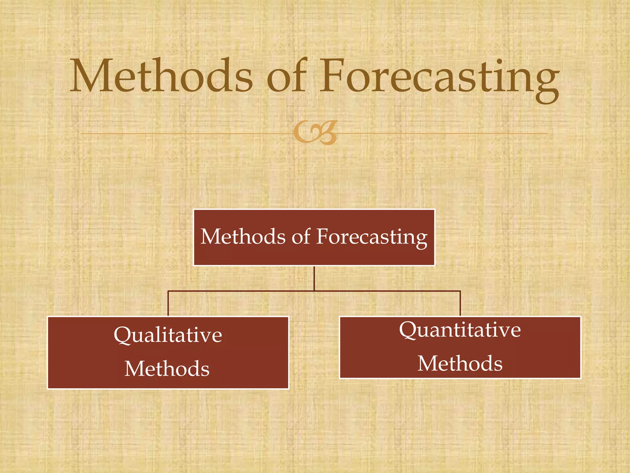
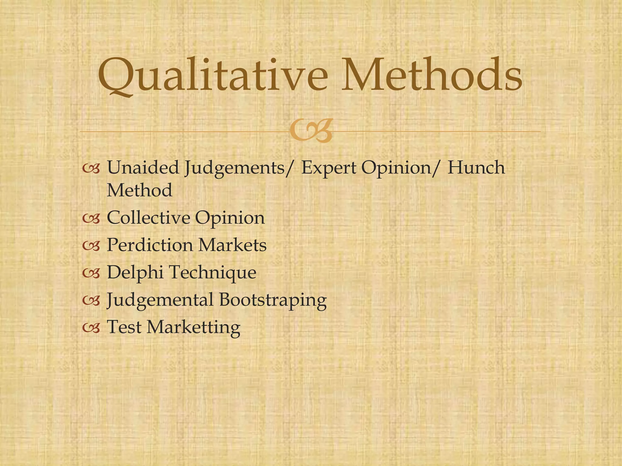
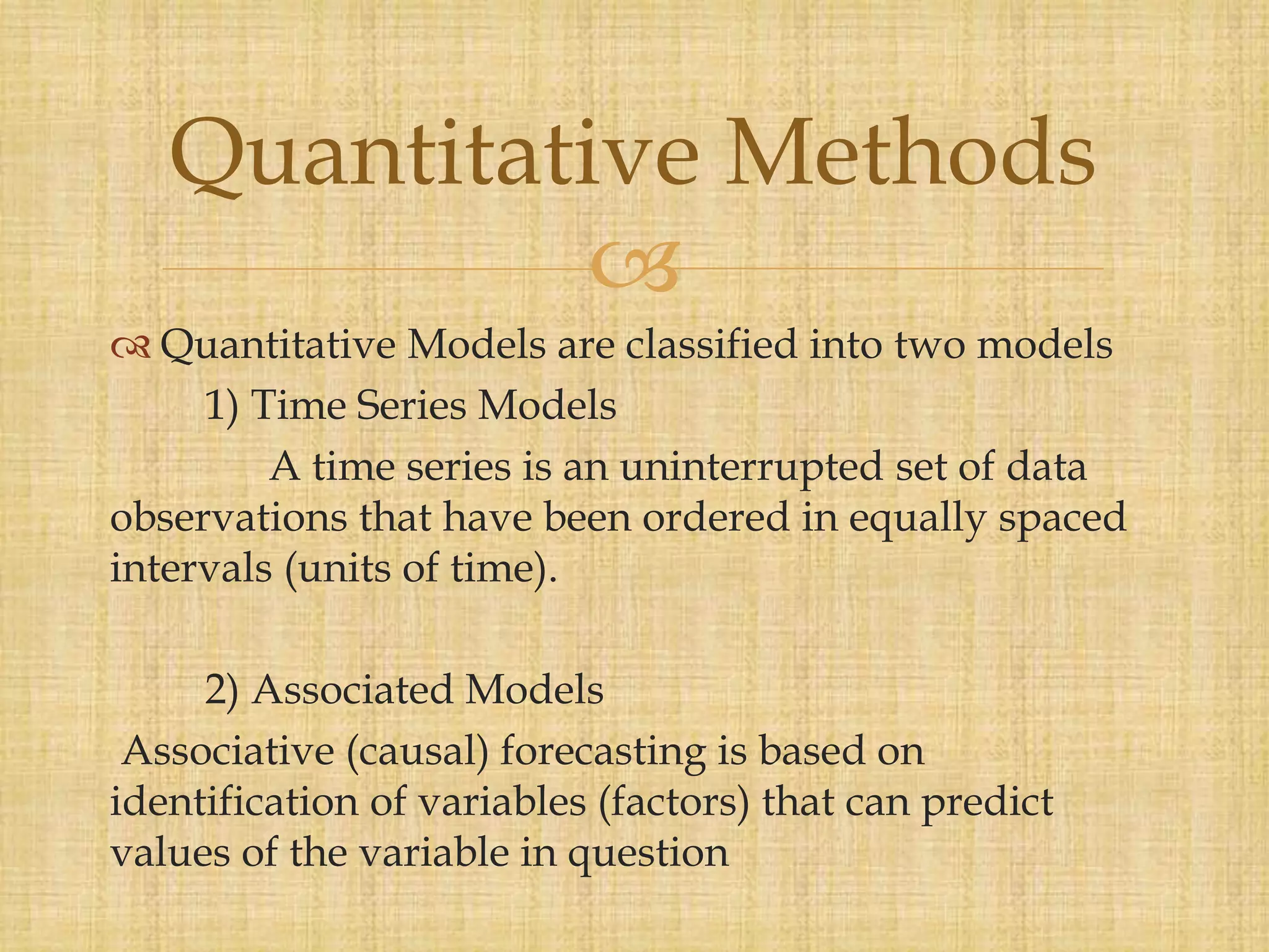
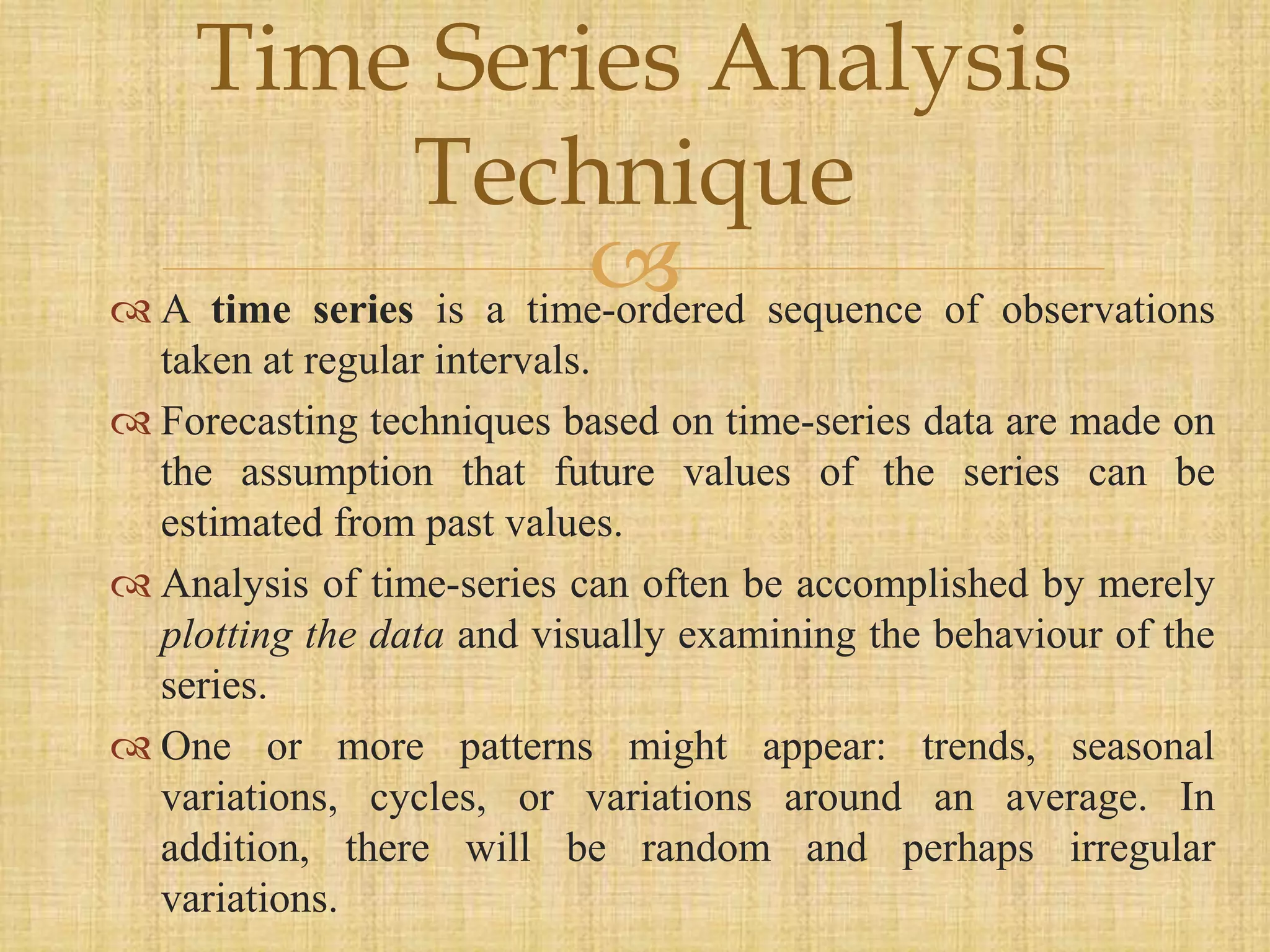
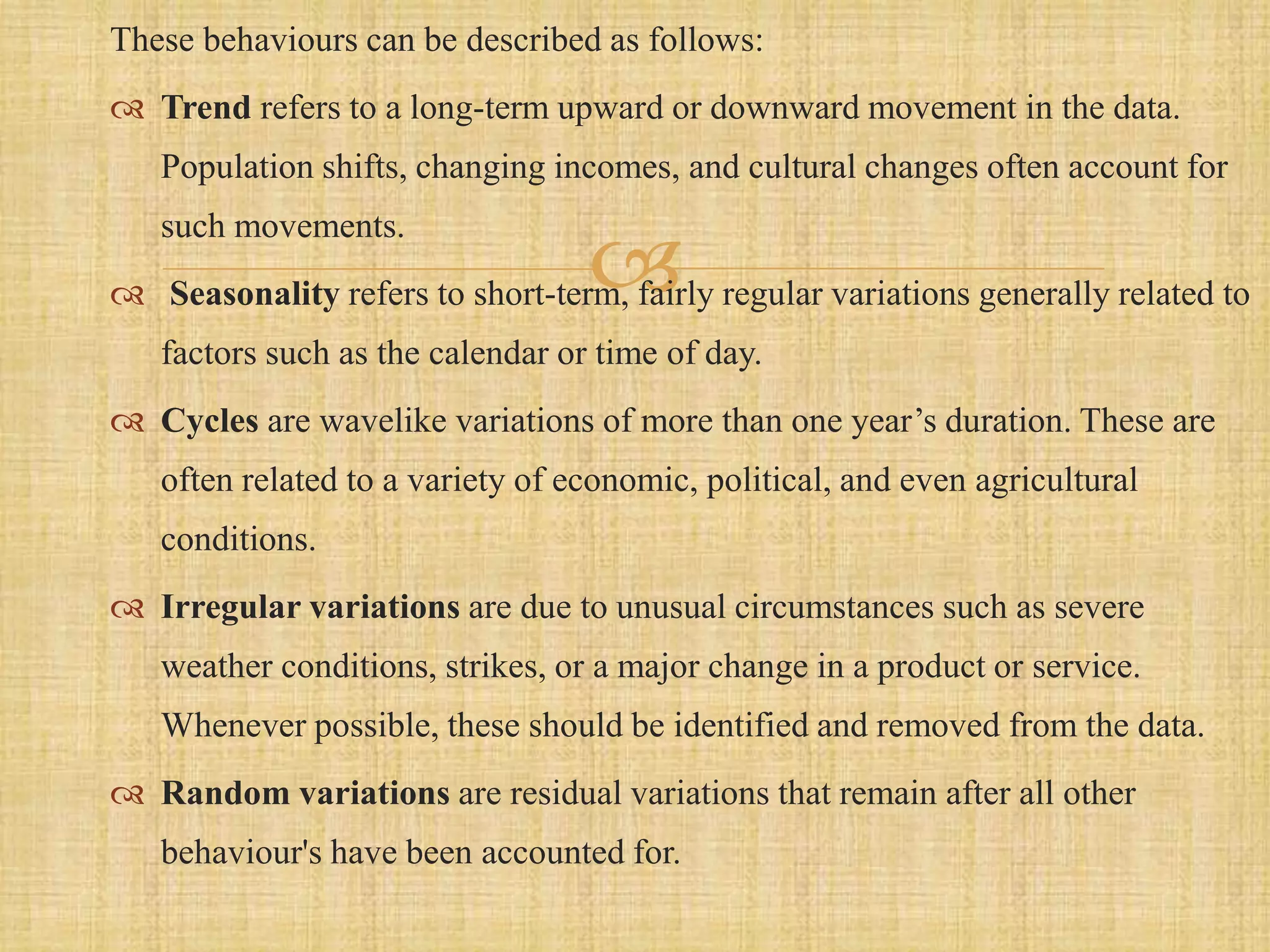
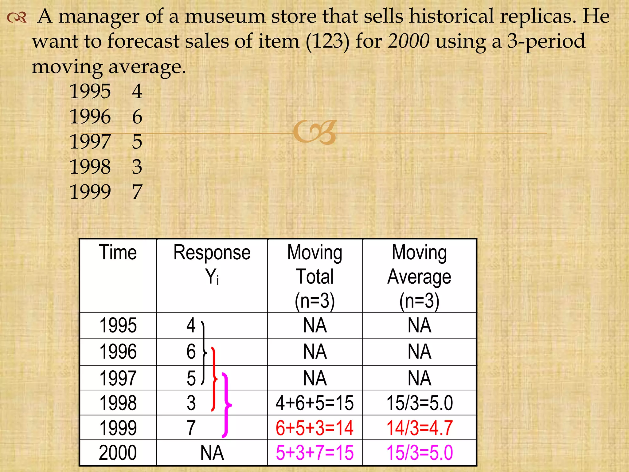
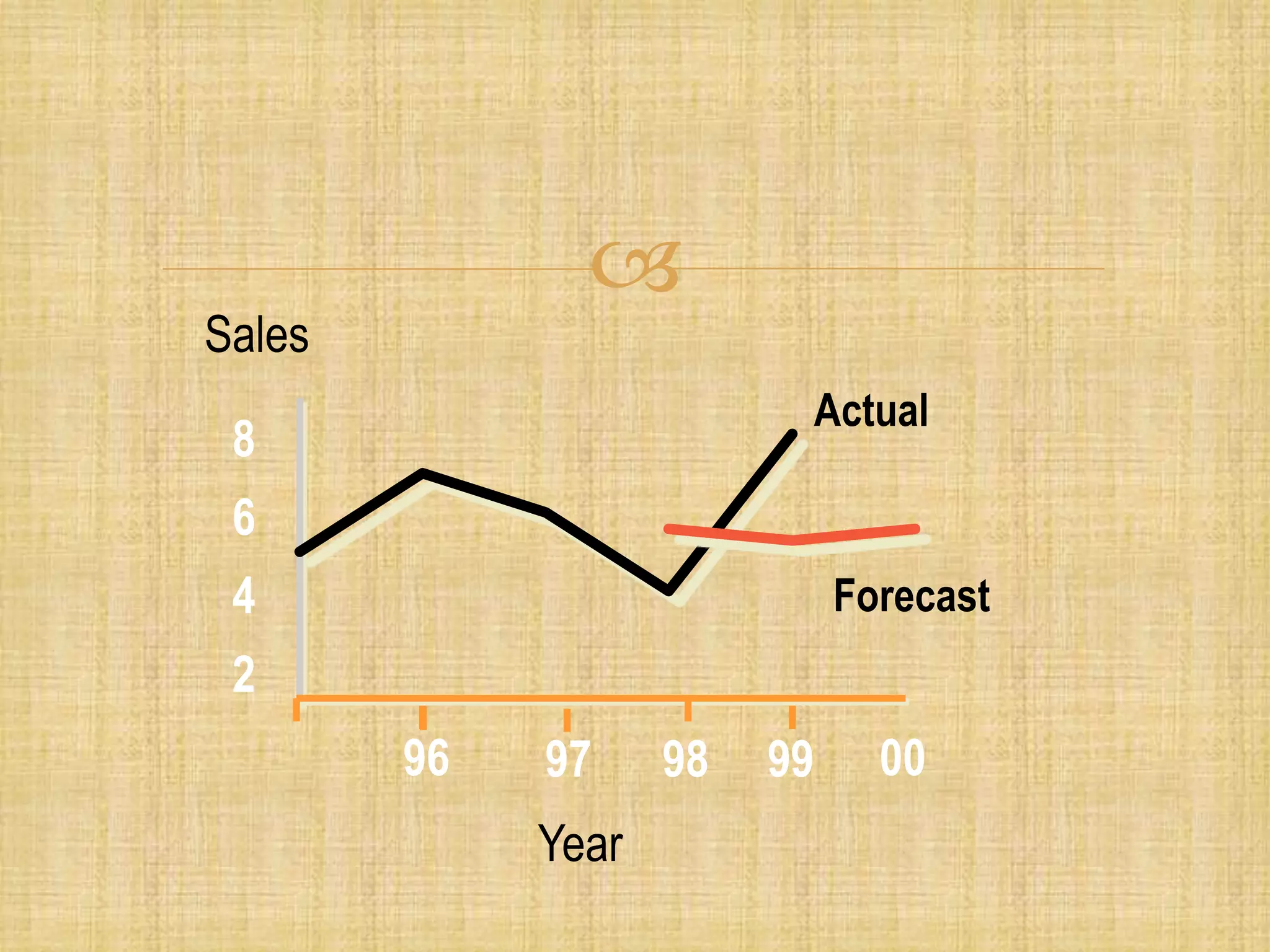
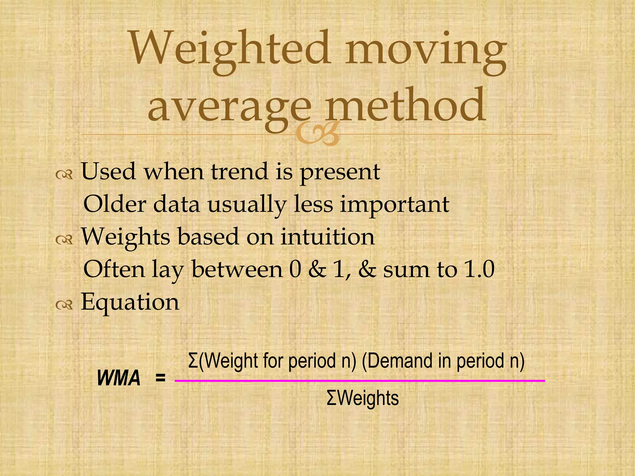
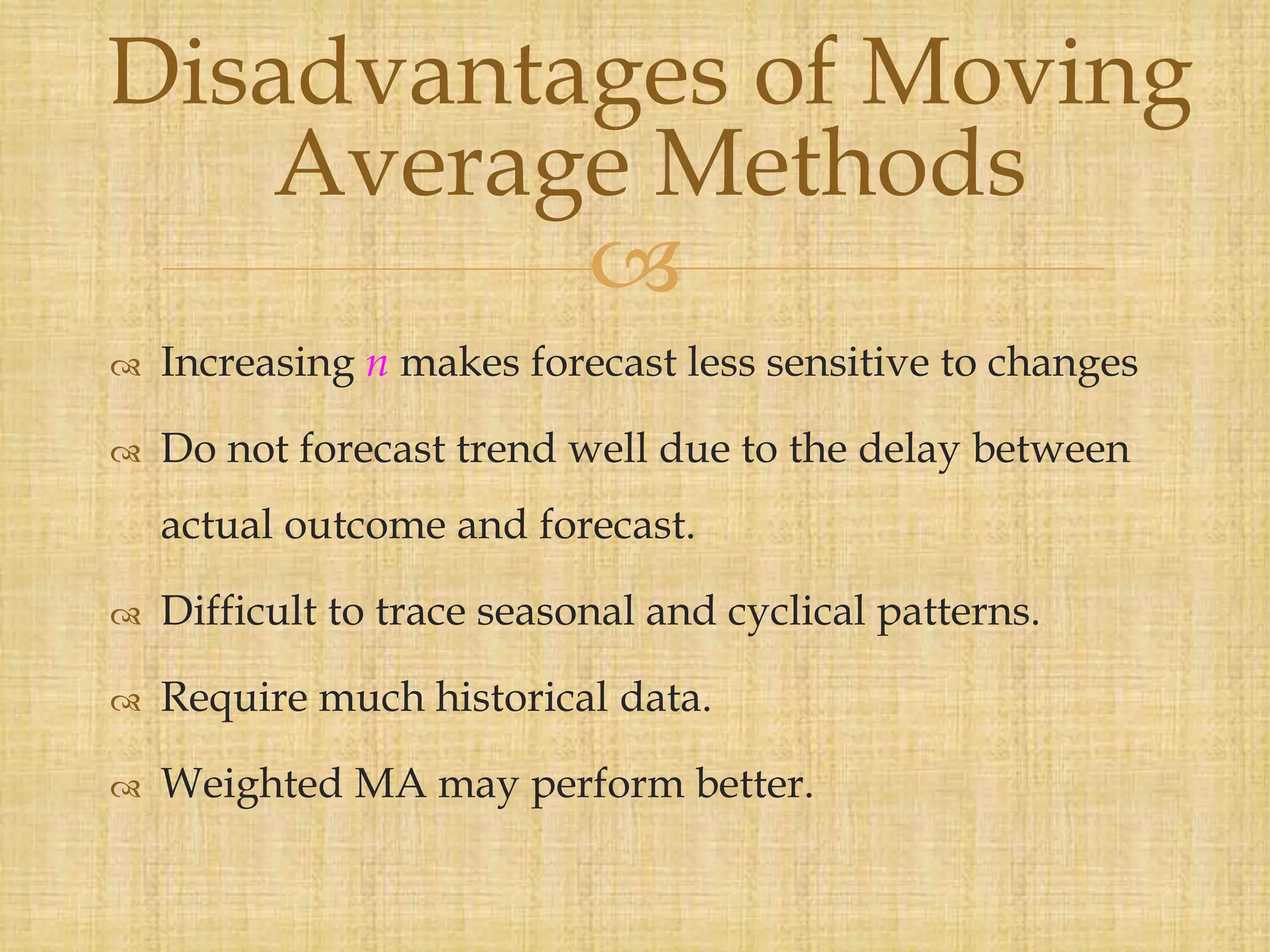
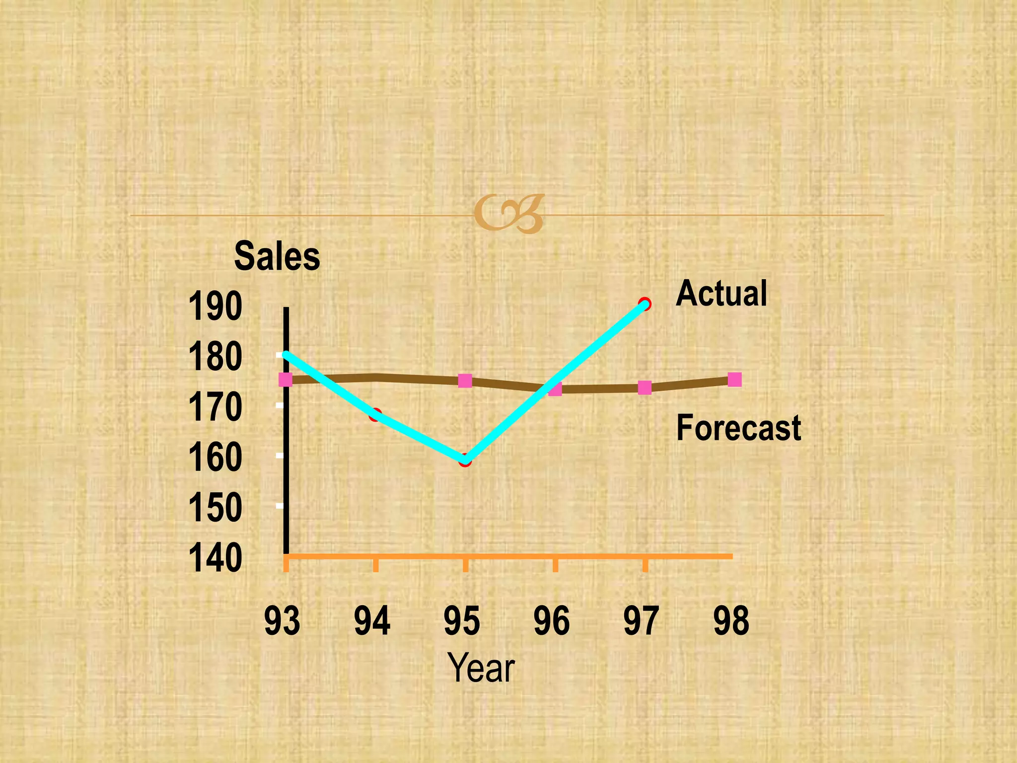
Milind A. Pelagade

 Forecasting is a process of estimating a future event
by casting forward past data.
 The past data are systematically combined in a
predetermined way to obtain the estimate of the
future.
 In business applications, forecasting serves as a
starting point of major decisions in finance,
marketing, productions, and purchasing.
Forecasting

Objective
 To predict demand for planning purposes
Laws of Forecasting
 Forecasts are always wrong.
 Forecasts always change.
 The further into the future, the less reliable the forecast will be.

 Determine the purpose of the forecast. How will it be used
and when will it be needed?
 Establish a time horizon. The forecast must indicate a time
interval, keeping in mind that accuracy decreases as the time
horizon increases.
 Obtain, clean, and analyse appropriate data. Obtaining the
data can involve significant effort. Once obtained, the data may
need to be “cleaned” to get rid of outliers and obviously
incorrect data before analysis.
 Select a forecasting technique.
 Make the forecast.
 Monitor the forecast. A forecast has to be monitored to
determine whether it is performing in a satisfactory manner.
Steps of Forecasting

Methods of Forecasting
Qualitative
Methods
Quantitative
Methods
Methods of Forecasting

 Unaided Judgements/ Expert Opinion/ Hunch
Method
 Collective Opinion
 Perdiction Markets
 Delphi Technique
 Judgemental Bootstraping
 Test Marketting
Qualitative Methods

 Quantitative Models are classified into two models
1) Time Series Models
A time series is an uninterrupted set of data
observations that have been ordered in equally spaced
intervals (units of time).
2) Associated Models
Associative (causal) forecasting is based on
identification of variables (factors) that can predict
values of the variable in question
Quantitative Methods
 A time series is a time-ordered sequence of observations
taken at regular intervals.
 Forecasting techniques based on time-series data are made on
the assumption that future values of the series can be
estimated from past values.
 Analysis of time-series can often be accomplished by merely
plotting the data and visually examining the behaviour of the
series.
 One or more patterns might appear: trends, seasonal
variations, cycles, or variations around an average. In
addition, there will be random and perhaps irregular
variations.
Time Series Analysis
Technique

These behaviours can be described as follows:
 Trend refers to a long-term upward or downward movement in the data.
Population shifts, changing incomes, and cultural changes often account for
such movements.
 Seasonality refers to short-term, fairly regular variations generally related to
factors such as the calendar or time of day.
 Cycles are wavelike variations of more than one year’s duration. These are
often related to a variety of economic, political, and even agricultural
conditions.
 Irregular variations are due to unusual circumstances such as severe
weather conditions, strikes, or a major change in a product or service.
Whenever possible, these should be identified and removed from the data.
 Random variations are residual variations that remain after all other
behaviour's have been accounted for.
 A trend line fitted to historical data points can project into the
medium to long-range
 Linear trends can be found using the least squares technique
y = a + bx
Where,
y= computed value of the variable to be predicted (dependent
variable)
a= y-axis intercept
b= slope of the regression line
x= the independent variable
Estimated by least squares method
Linear Regression

 Criteria of finding a and b:
Equation: ii bxaY ˆ
Slope: 22
1
1
xnx
yxnyx
b
i
n
i
ii
n
i





Y-Intercept: xbya 
 MA is a series of arithmetic means
 Used if little or no trend, seasonal, and
cyclical patterns
 Used often for smoothing
 Provides overall impression of data over
time
Equation,
Simple Moving Average
Method
MA
n
n
  Demand in Previous Periods

 A manager of a museum store that sells historical replicas. He
want to forecast sales of item (123) for 2000 using a 3-period
moving average.
1995 4
1996 6
1997 5
1998 3
1999 7
Time Response
Yi
Moving
Total
(n=3)
Moving
Average
(n=3)
1995 4 NA NA
1996 6 NA NA
1997 5 NA NA
1998 3 4+6+5=15 15/3=5.0
1999 7 6+5+3=14 14/3=4.7
2000 NA 5+3+7=15 15/3=5.0

Year
Sales
2
4
6
8
Actual
Forecast
96 97 98 99 00

 Used when trend is present
Older data usually less important
 Weights based on intuition
Often lay between 0 & 1, & sum to 1.0
 Equation
Weighted moving
average method
WMA =
Σ(Weight for period n) (Demand in period n)
ΣWeights

 Increasing n makes forecast less sensitive to changes
 Do not forecast trend well due to the delay between
actual outcome and forecast.
 Difficult to trace seasonal and cyclical patterns.
 Require much historical data.
 Weighted MA may perform better.
Disadvantages of Moving
Average Methods

 Form of weighted moving average
 Weights decline exponentially
 Most recent data weighted most
 This method requires only the current demand and forecast
demand.
 This method assigns weight to all the previous data.
 The reason this is called exponential smoothing is that
each increment in the past is decreased by (1-α).
Exponential Smoothing
Method

 Ft = Ft-1 + (At-1 - Ft-1)
= At-1 + (1 - ) Ft-1
Ft = Forecast value
At = Actual value
 = Smoothing constant

Suppose you are organizing a Kwanza meeting. You want to
forecast attendance for 2000 using exponential smoothing
( = .10). The 1995 (made in 1994) forecast was 175.
Actual data:
1995 180
1996 168
1997 159
1998 175
1999 190

Time Actual
Forecast,
(α = .10)
1995 180
1996 168 175.00 + .10(180 - 175.00) = 175.50
1997 159 175.50 + .10(168 - 175.50) = 174.75
1998 175 174.75 + .10(159 - 174.75) = 173.18
1999 190 173.18 + .10(175 - 173.18) = 173.36
2000 173.36 + .10(190 - 173.36) = 175.02
Ft = Ft-1 +  · (At-1 - Ft-1)
NA
175(Given)

Year
Sales
140
150
160
170
180
190
93 94 95 96 97 98
Actual
Forecast

 Why Causal Forecasting ?
 There is no logical link between the demand in the
future and what has happened in the past
 There are other factors which can be logically linked to
the demand
 Example 1: There is a strong cause and effect
relationship between future demand for doors and
windows and the number of construction permits
issued at present.
 Example 2: The demand for new house or automobile is
very much affected by the interest rates changed by
banks.
Casual method


Forecasting and methods of forecasting

  • 1.
  • 2.
      Forecasting isa process of estimating a future event by casting forward past data.  The past data are systematically combined in a predetermined way to obtain the estimate of the future.  In business applications, forecasting serves as a starting point of major decisions in finance, marketing, productions, and purchasing. Forecasting
  • 3.
     Objective  To predictdemand for planning purposes Laws of Forecasting  Forecasts are always wrong.  Forecasts always change.  The further into the future, the less reliable the forecast will be.
  • 4.
  • 5.
     Determine thepurpose of the forecast. How will it be used and when will it be needed?  Establish a time horizon. The forecast must indicate a time interval, keeping in mind that accuracy decreases as the time horizon increases.  Obtain, clean, and analyse appropriate data. Obtaining the data can involve significant effort. Once obtained, the data may need to be “cleaned” to get rid of outliers and obviously incorrect data before analysis.  Select a forecasting technique.  Make the forecast.  Monitor the forecast. A forecast has to be monitored to determine whether it is performing in a satisfactory manner. Steps of Forecasting
  • 6.
  • 7.
      Unaided Judgements/Expert Opinion/ Hunch Method  Collective Opinion  Perdiction Markets  Delphi Technique  Judgemental Bootstraping  Test Marketting Qualitative Methods
  • 8.
      Quantitative Modelsare classified into two models 1) Time Series Models A time series is an uninterrupted set of data observations that have been ordered in equally spaced intervals (units of time). 2) Associated Models Associative (causal) forecasting is based on identification of variables (factors) that can predict values of the variable in question Quantitative Methods
  • 9.
     A timeseries is a time-ordered sequence of observations taken at regular intervals.  Forecasting techniques based on time-series data are made on the assumption that future values of the series can be estimated from past values.  Analysis of time-series can often be accomplished by merely plotting the data and visually examining the behaviour of the series.  One or more patterns might appear: trends, seasonal variations, cycles, or variations around an average. In addition, there will be random and perhaps irregular variations. Time Series Analysis Technique
  • 10.
     These behaviours canbe described as follows:  Trend refers to a long-term upward or downward movement in the data. Population shifts, changing incomes, and cultural changes often account for such movements.  Seasonality refers to short-term, fairly regular variations generally related to factors such as the calendar or time of day.  Cycles are wavelike variations of more than one year’s duration. These are often related to a variety of economic, political, and even agricultural conditions.  Irregular variations are due to unusual circumstances such as severe weather conditions, strikes, or a major change in a product or service. Whenever possible, these should be identified and removed from the data.  Random variations are residual variations that remain after all other behaviour's have been accounted for.
  • 11.
     A trendline fitted to historical data points can project into the medium to long-range  Linear trends can be found using the least squares technique y = a + bx Where, y= computed value of the variable to be predicted (dependent variable) a= y-axis intercept b= slope of the regression line x= the independent variable Estimated by least squares method Linear Regression
  • 12.
      Criteria offinding a and b: Equation: ii bxaY ˆ Slope: 22 1 1 xnx yxnyx b i n i ii n i      Y-Intercept: xbya 
  • 13.
     MA isa series of arithmetic means  Used if little or no trend, seasonal, and cyclical patterns  Used often for smoothing  Provides overall impression of data over time Equation, Simple Moving Average Method MA n n   Demand in Previous Periods
  • 14.
      A managerof a museum store that sells historical replicas. He want to forecast sales of item (123) for 2000 using a 3-period moving average. 1995 4 1996 6 1997 5 1998 3 1999 7 Time Response Yi Moving Total (n=3) Moving Average (n=3) 1995 4 NA NA 1996 6 NA NA 1997 5 NA NA 1998 3 4+6+5=15 15/3=5.0 1999 7 6+5+3=14 14/3=4.7 2000 NA 5+3+7=15 15/3=5.0
  • 15.
  • 16.
      Used whentrend is present Older data usually less important  Weights based on intuition Often lay between 0 & 1, & sum to 1.0  Equation Weighted moving average method WMA = Σ(Weight for period n) (Demand in period n) ΣWeights
  • 17.
      Increasing nmakes forecast less sensitive to changes  Do not forecast trend well due to the delay between actual outcome and forecast.  Difficult to trace seasonal and cyclical patterns.  Require much historical data.  Weighted MA may perform better. Disadvantages of Moving Average Methods
  • 18.
      Form ofweighted moving average  Weights decline exponentially  Most recent data weighted most  This method requires only the current demand and forecast demand.  This method assigns weight to all the previous data.  The reason this is called exponential smoothing is that each increment in the past is decreased by (1-α). Exponential Smoothing Method
  • 19.
      Ft =Ft-1 + (At-1 - Ft-1) = At-1 + (1 - ) Ft-1 Ft = Forecast value At = Actual value  = Smoothing constant
  • 20.
     Suppose you areorganizing a Kwanza meeting. You want to forecast attendance for 2000 using exponential smoothing ( = .10). The 1995 (made in 1994) forecast was 175. Actual data: 1995 180 1996 168 1997 159 1998 175 1999 190
  • 21.
     Time Actual Forecast, (α =.10) 1995 180 1996 168 175.00 + .10(180 - 175.00) = 175.50 1997 159 175.50 + .10(168 - 175.50) = 174.75 1998 175 174.75 + .10(159 - 174.75) = 173.18 1999 190 173.18 + .10(175 - 173.18) = 173.36 2000 173.36 + .10(190 - 173.36) = 175.02 Ft = Ft-1 +  · (At-1 - Ft-1) NA 175(Given)
  • 22.
  • 23.
      Why CausalForecasting ?  There is no logical link between the demand in the future and what has happened in the past  There are other factors which can be logically linked to the demand  Example 1: There is a strong cause and effect relationship between future demand for doors and windows and the number of construction permits issued at present.  Example 2: The demand for new house or automobile is very much affected by the interest rates changed by banks. Casual method
  • 24.