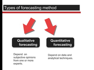
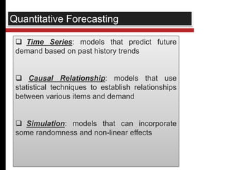
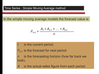
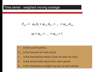
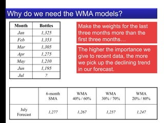
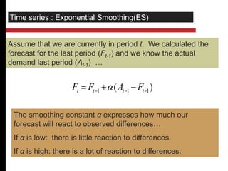
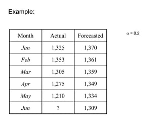
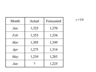
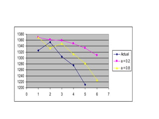
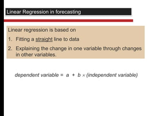
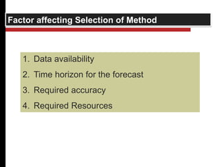
Quantitative Forecasting 
Prepared By :- 
Jaydeep Kanetiya 
Loriya Ravi
What is Forecasting ? 
 Forecasting is a tool used for predicting future 
Forecasting Forecasting is is a a tool tool used used for for predicting 
predicting 
demand based on past demand information. 
future demand based on 
past demand information. 
future demand based on 
past demand information. 
Forecasting is a tool used for predicting 
 A forecast is only as good as the information 
included in the forecast (past data) 
future demand based on 
past demand information. 
 Forecasting is based on the assumption that the past 
predicts the future!
Types of forecasting method 
Qualitative 
forecasting 
Quantitative 
forecasting 
Depend on 
subjective opinions 
from one or more 
experts. 
Depend on data and 
analytical techniques.
Quantitative Forecasting 
 Time Series: models that predict future 
demand based on past history trends 
 Causal Relationship: models that use 
statistical techniques to establish relationships 
between various items and demand 
 Simulation: models that can incorporate 
some randomness and non-linear effects
Time Series : Simple Moving Average method 
In the simple moving average models the forecast value is 
At + At-1 + … + At-n 
Ft+1 = ------------------------------- 
n 
t is the current period. 
Ft+1 is the forecast for next period 
n is the forecasting horizon (how far back we 
look), 
A is the actual sales figure from each period.
A 
B 
C 
D 
E 
F 
G 
H 
I 
J 
K 
L 
M 
N 
O 
P 
E 
R 
T 
T 
Y 
D 
g 
e 
Example: forecasting sales at Coca-Cola 
Month Bottles 
Jan 1,325 
Feb 1,353 
Mar 1,305 
Apr 1,275 
May 1,210 
Jun 1,195 
Jul ?
A 
B 
C 
D 
E 
F 
G 
H 
I 
J 
K 
L 
M 
N 
O 
P 
E 
R 
T 
T 
Y 
D 
g 
e 
What if we use a 3-month simple moving average? 
AJun + AMay + AApr 
FJul = ---------------------------- 
3 
= 1,227 
What if we use a 5-month simple moving average? 
AJun + AMay + AApr + AMar + AFeb 
FJul = ------------------------------------------ 
5 
= 1,268
A 
B 
C 
D 
E 
F 
G 
H 
I 
J 
K 
L 
M 
N 
O 
P 
E 
R 
T 
T 
Y 
D 
g 
e 
1400 
1350 
1300 
1250 
1200 
1150 
1100 
1050 
1000 
0 1 2 3 4 5 6 7 8 
5-month 
MA forecast 
3-month 
MA forecast 
What do we observe? 
5-month average smoothes data more; 
3-month average more responsive
Time series : weighted moving average 
Ft+1 = wt At + wt-1 At-1 + … + wt-n At-n 
wt + wt-1 + … + wt-n = 1 
t is the current period. 
Ft+1 is the forecast for next period 
n is the forecasting horizon (how far back we look), 
A is the actual sales figure from each period. 
w is the importance (weight) we give to each period
A 
B 
C 
D 
E 
F 
G 
H 
I 
J 
K 
L 
M 
N 
O 
P 
E 
R 
T 
T 
Y 
D 
g 
e 
Why do we need the WMA models? 
Month Bottles 
Jan 1,325 
Feb 1,353 
Mar 1,305 
Apr 1,275 
May 1,210 
Jun 1,195 
Jul ? 
Make the weights for the last 
three months more than the 
first three months… 
6-month 
SMA 
The higher the importance we 
give to recent data, the more 
we pick up the declining trend 
in our forecast. 
WMA 
40% / 60% 
WMA 
30% / 70% 
WMA 
20% / 80% 
July 
Forecast 
1,277 1,267 1,257 1,247
Time series : Exponential Smoothing(ES) 
Assume that we are currently in period t. We calculated the 
forecast for the last period (Ft-1) and we know the actual 
demand last period (At-1) … 
( ) 1 1 1    t t t t F F  A F 
The smoothing constant α expresses how much our 
forecast will react to observed differences… 
If α is low: there is little reaction to differences. 
If α is high: there is a lot of reaction to differences.
Example: 
Month Actual Forecasted 
Jan 1,325 1,370 
Feb 1,353 1,361 
Mar 1,305 1,359 
Apr 1,275 1,349 
May 1,210 1,334 
Jun ? 1,309 
 = 0.2
Month Actual Forecasted 
Jan 1,325 1,370 
Feb 1,353 1,334 
Mar 1,305 1,349 
Apr 1,275 1,314 
May 1,210 1,283 
Jun ? 1,225 
 = 0.8
1380 
1360 
1340 
1320 
1300 
1280 
1260 
1240 
1220 
1200 
0 1 2 3 4 5 6 7 
Actual 
a = 0.2 
a = 0.8
Linear Regression in forecasting 
Linear regression is based on 
1. Fitting a straight line to data 
2. Explaining the change in one variable through changes 
in other variables. 
dependent variable = a + b  (independent variable)
Factor affecting Selection of Method 
1. Data availability 
2. Time horizon for the forecast 
3. Required accuracy 
4. Required Resources
References 
www.csb.uncw.edu 
www.prism.gatech.edu 
web.calstatela.edu 
www.forecasters.org 
www.csun.edu
Quantitative forecasting

Quantitative forecasting

  • 1.
    Quantitative Forecasting PreparedBy :- Jaydeep Kanetiya Loriya Ravi
  • 2.
    What is Forecasting?  Forecasting is a tool used for predicting future Forecasting Forecasting is is a a tool tool used used for for predicting predicting demand based on past demand information. future demand based on past demand information. future demand based on past demand information. Forecasting is a tool used for predicting  A forecast is only as good as the information included in the forecast (past data) future demand based on past demand information.  Forecasting is based on the assumption that the past predicts the future!
  • 3.
    Types of forecastingmethod Qualitative forecasting Quantitative forecasting Depend on subjective opinions from one or more experts. Depend on data and analytical techniques.
  • 4.
    Quantitative Forecasting Time Series: models that predict future demand based on past history trends  Causal Relationship: models that use statistical techniques to establish relationships between various items and demand  Simulation: models that can incorporate some randomness and non-linear effects
  • 5.
    Time Series :Simple Moving Average method In the simple moving average models the forecast value is At + At-1 + … + At-n Ft+1 = ------------------------------- n t is the current period. Ft+1 is the forecast for next period n is the forecasting horizon (how far back we look), A is the actual sales figure from each period.
  • 6.
    A B C D E F G H I J K L M N O P E R T T Y D g e Example: forecasting sales at Coca-Cola Month Bottles Jan 1,325 Feb 1,353 Mar 1,305 Apr 1,275 May 1,210 Jun 1,195 Jul ?
  • 7.
    A B C D E F G H I J K L M N O P E R T T Y D g e What if we use a 3-month simple moving average? AJun + AMay + AApr FJul = ---------------------------- 3 = 1,227 What if we use a 5-month simple moving average? AJun + AMay + AApr + AMar + AFeb FJul = ------------------------------------------ 5 = 1,268
  • 8.
    A B C D E F G H I J K L M N O P E R T T Y D g e 1400 1350 1300 1250 1200 1150 1100 1050 1000 0 1 2 3 4 5 6 7 8 5-month MA forecast 3-month MA forecast What do we observe? 5-month average smoothes data more; 3-month average more responsive
  • 9.
    Time series :weighted moving average Ft+1 = wt At + wt-1 At-1 + … + wt-n At-n wt + wt-1 + … + wt-n = 1 t is the current period. Ft+1 is the forecast for next period n is the forecasting horizon (how far back we look), A is the actual sales figure from each period. w is the importance (weight) we give to each period
  • 10.
    A B C D E F G H I J K L M N O P E R T T Y D g e Why do we need the WMA models? Month Bottles Jan 1,325 Feb 1,353 Mar 1,305 Apr 1,275 May 1,210 Jun 1,195 Jul ? Make the weights for the last three months more than the first three months… 6-month SMA The higher the importance we give to recent data, the more we pick up the declining trend in our forecast. WMA 40% / 60% WMA 30% / 70% WMA 20% / 80% July Forecast 1,277 1,267 1,257 1,247
  • 11.
    Time series :Exponential Smoothing(ES) Assume that we are currently in period t. We calculated the forecast for the last period (Ft-1) and we know the actual demand last period (At-1) … ( ) 1 1 1    t t t t F F  A F The smoothing constant α expresses how much our forecast will react to observed differences… If α is low: there is little reaction to differences. If α is high: there is a lot of reaction to differences.
  • 12.
    Example: Month ActualForecasted Jan 1,325 1,370 Feb 1,353 1,361 Mar 1,305 1,359 Apr 1,275 1,349 May 1,210 1,334 Jun ? 1,309  = 0.2
  • 13.
    Month Actual Forecasted Jan 1,325 1,370 Feb 1,353 1,334 Mar 1,305 1,349 Apr 1,275 1,314 May 1,210 1,283 Jun ? 1,225  = 0.8
  • 14.
    1380 1360 1340 1320 1300 1280 1260 1240 1220 1200 0 1 2 3 4 5 6 7 Actual a = 0.2 a = 0.8
  • 15.
    Linear Regression inforecasting Linear regression is based on 1. Fitting a straight line to data 2. Explaining the change in one variable through changes in other variables. dependent variable = a + b  (independent variable)
  • 16.
    Factor affecting Selectionof Method 1. Data availability 2. Time horizon for the forecast 3. Required accuracy 4. Required Resources
  • 17.
    References www.csb.uncw.edu www.prism.gatech.edu web.calstatela.edu www.forecasters.org www.csun.edu